Principles of Nutritional Assessment:

Nutritional Assessment: Introduction

Nutritional assessment procedures were first used in surveys designed to describe the nutritional status of populations on a national basis. The assessment methods used were initially described following a conference held in 1932 by the Health Organization of the League of Nations.

In 1955, the Interdepartmental Committee on Nutrition for National Defense (ICNND) was organized to assist low-income countries in assessing the nutritional status of their populations and to identify problems of malnu­trition and the ways in which they could be solved. The ICNND teams conducted medical nutri­tion surveys in 24 countries. A comprehensive manual was then produced and later, updated guidance issued (ICNND, 1984) with the intention of standardizing both the assessment methods used for the collection of nutri­tion survey data and the inter­pretation of the results.

On the recom­men­dation of a World Health Organization (WHO) Expert Committee on Medical assessment of Nutritional Status, a second publication was prepared by Jelliffe (1966) in consultation with 25 specialists from various countries. This monograph was directed specifically at the assessment of the nutritional status of vulnerable groups in low-income countries of the world.

Many of the methods described in this monograph are still used by the the U.S. Demographic and Health Surveys (DHS) Program to collect representative data on popu­lation, health, HIV, and nutri­tion, and about 30 indicators supporting the Sustainable Development Goals. The data are used to identify public health nutri­tion problems so that effective inter­vention programs can be designed. The U.S. DHS program has conducted more than 400 surveys in over 90 low‑ and middle-income countries since 1984.

Many higher income countries collect national data on the nutritional status of the popu­lation, some (e.g., the U.S. and the U.K.) collecting data on an ongoing basis using nutri­tion surveillance systems. In the past, these systems have often targeted high-risk populations, especially low-income mothers, children under five, and pregnant women. Now, with the growing awareness of the role of nutri­tion as a risk factor for chronic diseases, surveillance systems often encompass all age groups.

1.0 New developments in nutritional assessment

Today, nutritional assessment emphasizes new simple non­invasive approaches, particularly valuable in low income countries, that can measure the risk of nutrient deficits and excesses, and monitor and evaluate the effects of nutri­tion inter­ventions. These new approaches to assessment include the measure­ment of nutrients and bio­markers in dried blood spots prepared from a finger-prick blood sample, avoiding the necessity for venous blood collection and refrigerated storage (Mei et al., 2001). In addition, for some nutrients, on-site analysis is now possible, enabling researchers and respondents to obtain results immediately.

Many of these new approaches can also be applied to bio­markers monitoring the risk of chronic diseases. These include bio­markers of antioxidant protection, soft-tissue oxidation, and free-radical formation, all of which have numerous clinical applications.

Increasingly, “all-in-one” instrumental platforms for multiple micro­nutrient tests on a single sample aliquot are being developed, some of which have been adapted for dried blood spot matrices (Brindle et al., 2019). These assessment instruments are designed so they are of low complexity and can be operated by labora­tory technicians with minimal training, making them especially useful in low- and middle-income countries (Esmaeili et al., 2019).

The public availability of e‑ and m‑Health communication technologies has increased dramatically in recent years. e‑Health is defined as:

“the use of emerging infor­mation and communications technology, especially the internet, to improve or enable health and health care”

whereas m-Health inter­ventions are

“those designed for delivery through mobile phones” (Olson, 2016).

Inter­ventions using these communication technologies to assess, monitor and improve nutri­tion-related behaviors and body weight, appear to be efficacious across cognitive outcomes, and some behavioral and emotional outcomes, although changing dietary behaviors is a more challenging outcome. There is an urgent need for a rigorous scientific evaluation of e‑ and m‑health inter­vention technologies. To date their public health impact remains uncertain.

Nutritional assessment is also an essential component of the nutritional care of the hospitalized patient. The important relationship between nutritional status and health, and particularly the critical role of nutri­tion in recovery from acute illness or injury, is well documented. Although it is many years since the preva­lence of malnu­trition among hospitalized patients was first reported (Bistrian et al., 1974, 1976), such malnu­trition still persists (Barker et al., 2011).

In the early 1990s, evidence-based medicine started as a movement in an effort to optimize clinical care. Originally, evidence-based-medicine focused on critical appraisal, followed by the development of methods and techniques for generating system­atic reviews and clinical practice guidelines (Djulbegovic and Guyatt, 2017). For more details see Section 1.1.6.

Point of care technology (POCT) is also a rapidly expanding health care approach that can be used in diverse settings, particularly those with limited health services or labora­tory infra­structure, as the tests do not require specialized equip­ment and are simple to use. The tests are also quick, enabling prompt clinical decisions to be made to improve the patient’s health at or near the site of patient care. The development and evaluation of POC devices for the diagnosis of malaria, tuberculosis, HIV, and other infectious diseases is on-going and holds promise for low-resource settings (Heidt et al., 2020; Mitra and Sharma, 2021). Guidelines by WHO (2019) for the development of POC devices globally are avail­able, but challenges with regulatory approval, quality assurance programs, and product service and support remain (Drain et al., 2014).

Personalized nutri­tion is also a rapidly expanding approach that tailors dietary recom­men­dation to the specific biological requirements of an individual on the basis of their health status and performance goals. See Setion 1.1.5 for more details. The approach has become possible with the increasing advances in “‑omic sciences” (e.g., nutri­genomics, proteomics and meta­bol­omics). See Chapter 15 and van Ommen et al. (2017) for more details.

Health-care administrators and the community in general, continue to demand demon­strable benefits from the investment of public funds in nutri­tion inter­vention programs. This requires improved techniques in nutritional assessment and the monitoring and evaluation of nutrition inter­ventions. In addition, implementation research is now being recognized as critical for maximizing the benefits of evidence-based inter­ventions. Implementation research in nutri­tion aims to build evidence-based knowledge and sound theory to design and implement programs that will deliver nutri­tion programs effectively. However, to overcome the unique challenges faced during the implementation of nutri­tion and health inter­ventions, strengthening the capacity of practitioners alongside that of health researchers is essential. Dako-Gyke et al. (2020) have developed an implementation research course curriculum that targets both practitioners and researchers simultaneously, and which is focused on low‑ and middle-income countries.

The aim of this 3^rd edition of “Principles of Nutritional assessment” is to provide guidance on some of these new, improved techniques, as well as a comprehensive and critical appraisal of many of the classic, well-established methods in nutritional assessment.

1.1 Nutritional assessment systems

Nutritional assessment systems involve the inter­pretation of infor­mation from dietary and nutritional bio­markers, and anthro­pometric and clinical studies. The infor­mation is used to determine the nutritional status of individuals or popu­lation groups as influenced by the intake and utilization of dietary substances and nutrients required to support growth, repair, and maintenance of the body as a whole or in any of its parts (Raiten and Combs, 2015).

Nutritional assessment systems can take one of four forms: surveys, surveillance, screening, or inter­ventions. These are described briefly below.

1.1.1 Nutrition surveys

The nutritional status of a selected popu­lation group is often assessed by means of a cross-sectional survey. The survey may either establish baseline nutritional data or ascertain the overall nutritional status of the popu­lation. Cross-sectional nutri­tion surveys can be used to examine associations, and to identify and describe popu­lation subgroups “at risk” for chronic malnu­trition. Causal relation­ships cannot be established from cross-sectional surveys because whether the exposure precedes or follows the effect is unknown. They are also unlikely to identify acute malnu­trition because all the measure­ments are taken on a single occasion or within a short time period with no follow-up. Nevertheless, infor­mation on preva­lence, defined as the proportion who have a condition or disease at one time point, can be obtained from cross-sectional surveys for use by health planners. Cross-sectional surveys are also a necessary and frequent first step in subsequent investigations into the causes of malnu­trition or disease.

National cross-sectional nutri­tion surveys generate valuable infor­mation on the preva­lence of existing health and nutritional problems in a country that can be used both to allocate resources to those popu­lation subgroups in need, and to formulate policies to improve the overall nutri­tion of the popu­lation. They are also sometimes used to evaluate nutri­tion inter­ventions by collecting baseline data before, and at the end of a nutri­tion inter­vention program, even though such a design is weak as the change may be attributable to some other factor (Section 1.1.4).

Several large-scale national nutri­tion surveys have been conducted in industrialized countries during the last decade. They include surveys in the United States, the United Kingdom, Ireland, New Zealand, and Australia. More than 400 Demo­graphic and Health Surveys (DHS) in over 90 low‑ and middle-income countries have also been completed. See U.S. DHS program.

1.1.2 Nutrition surveillance

The characteristic feature of surveillance is the continuous monitoring of the nutritional status of selected popu­lation groups. Surveillance studies therefore differ from nutri­tion surveys because the data are collected, analyzed, and utilized over an extended period of time. Sometimes, the surveillance only involves specific at‑risk subgroups, identified in earlier nutri­tion surveys.

The infor­mation collected from nutri­tion surveillance programs can be used to achieve the objec­tives shown in Box 1.1. Surveillance studies, unlike cross-sectional nutri­tion surveys, can also identify the possible causes of both chronic and acute malnu­trition and, hence, can be used to formulate and initiate inter­vention measures at either the popu­lation or the subpopulation level.

In the United States, a comprehensive program of national nutri­tion surveillance, known as the National Health and Nutrition Examination Survey (NHANES), has been conducted since 1959. Data on anthro­pometry, demographic and socio-economic status, dietary and health-related measures are collected. In 2008, the United Kingdom began the National Diet and Nutrition Survey Rolling Program. This is a continuous program of field work designed to assess the diet, nutrient intake, and nutritional status of the general popu­lation aged 1.5y and over living in private house­holds in the U.K. (Whitton et al., 2011). WHO has provided some countries with surveillance systems so that they can monitor changes in the global targets to reduce the high burden of disease asso­ciated with malnu­trition.

Note that the term “nutri­tion monitoring,” rather than nutri­tion surveillance, is often used when the partic­ipants selected are high‑risk individuals (e.g., food‑insecure house­holds, pregnant women). For example, because house­hold food insecurity is of increasing public health concern, even in high-income countries such as the U.S. and Canada, food insecurity is regularly monitored in these countries using the Household Food Security Survey Module (HFSSM). Also see: Loopstra (2018).

1.1.3 Nutrition screening

The identification of malnour­ished individuals requiring inter­vention can be accomplished by nutri­tion screening. This involves a comparison of measure­ments on individuals with pre­deter­mined risk levels or “cutoff” points using measure­ments that are accurate, simple and cheap (Section 1.5.3), and which can be applied rapidly on a large scale. Nutrition screening can be carried out on the whole popu­lation, targeted to a specific subpopulation considered to be at risk, or on selected individuals. The programs are usually less comprehensive than surveys or surveillance studies.

Numerous nutri­tion screening tools are avail­able for the early identification and treat­ment of malnu­trition in hospital patients and nursing homes, of which Subjective Global assessment (SGA) and the Malnutrition Universal Screening Tool (MUST) are widely used; see Barker et al. (2011) and Chapter 27 for more details.

In low-income countries, mid‑upper‑arm circum­ference (MUAC) with a fixed cutoff of 115mm is often used as screening tool to diagnose severe acute malnu­trition (SAM) in children aged 6–60mos (WHO/UNICEF, 2009). In some settings, mothers have been supplied with MUAC tapes either labeled with a specific cutoff of < 115mm, or color-coded in red (MUAC < 115mm), yellow (MUAC = 115–124mm), and green (MUAC > 125mm) in an effort to detect malnu­trition early, before the onset of complications, and thus reduce the need for inpatient treat­ment (Blackwell et al., 2015; Isanaka et al., 2020).

In the United States, screening is used to identify individuals who might benefit from the Supplemental Nutrition Assistance Program (SNAP). The program is means tested with highly selective qualifying criteria. The SNAP (formerly food stamps) program provides money loaded onto a payment card which can be used to purchase eligible foods, to ensure that eligible house­holds do not go without foods. In general, studies have reported that participation in SNAP is asso­ciated with a significant decline in food insecurity (Mabli and Ohls, 2015).

The U.S. also has a Special Supplemental Nutrition Program for Women, Infants, and Children (WIC) that targets low-income pregnant and post-partum women, infants, and children < 5y. In 2009, the USDA updated the WIC food packages in an effort to balance nutrient adequacy with reducing the risk of obesity; details of the updates are avail­able in NASEM (2006). Guthrie et al. (2020) compared associations between WIC partic­ipants and the nutrients and food packages consumed in 2008 and in 2016 using data from cross-sectional nationwide surveys of children aged < 4y. The findings indicated that more WIC infants who received the updated WIC food packages in 2016 had nutrient intakes (except iron) that met their estimated average requirements (EARs). Moreover, vegetables provided a larger contribution to their nutrient intakes, and intakes of low‑fat milks had increased for toddlers aged 2y, likely contributing to their lower reported intakes of saturated fat.

1.1.4 Nutrition inter­ventions

Nutrition inter­ventions often target popu­lation subgroups identified as “at‑risk” during nutri­tion surveys or by nutri­tion screening. In 2013, the Lancet Maternal and Child Nutrition Series recom­mended a package of nutri­tion inter­ventions that, if scaled to 90% coverage, could reduce stunting by 20% and reduce infant and child mortality by 15% (Bhutta et al., 2013). The nutri­tion inter­ventions considered included lipid-based and micro­nutrient supplementation, food fortification, promotion of exclusive breast feeding, dietary approaches, comple­mentary feeding, and nutri­tion education. More recently, nutri­tion inter­ventions that address nutri­tion-sensitive agriculture are also being extensively investigated (Sharma et al., 2021)

Increasingly, health-care program administrators and funding agencies are requesting evidence that inter­vention programs are implemented as planned, reach their target group in a cost-effective manner, and are having the desired impact. Hence, monitoring and evaluation are becoming an essential component of all nutri­tion inter­vention programs. However, because the etiology of malnu­trition is multi-factorial and requires a multi-sectorial response, the measure­ment and collection of the data from such multiple levels presents major challenges.

Several publications are avail­able on the design, monitoring, and evaluation of nutri­tion inter­ventions. The reader is advised to consult these sources for further details (Habicht et al., 1999; Rossi et al., 1999; Altman et al., 2001). Only a brief summary is given below.

Monitoring, discussed in detail by Levinson et al. (1999), oversees the implementation of an inter­vention, and can be used to assess service provision, utilization, coverage, and sometimes the cost of the program. Effective monitoring is essential to demonstrate that any observed result is probably from the inter­vention.

Emphasis on the importance of designing a program theory framework and asso­ciated program impact pathway (PIP) to understand and improve program delivery, utilization, and the potential of the program for nutritional impact has increased (Olney et al., 2013; Habicht and Pelto, 2019). The construction of a PIP helps conceptualize the program and its different components (i.e., inputs, processes, outputs, and outcomes to impacts). Only with this infor­mation can issues in program design, implementation, or utilization that may have the potential to limit the impact of the program, be identified, and, in turn strengthened, so the impact of the program can be optimized. Program impact pathway analysis generally includes both quantitative and qualitative methods (e.g., behavior-change communication) to ascertain the coverage of an inter­vention.

An example of the multiple levels of measure­ments and data that were collected to optimize the impact of a “Homestead Food Production” program conducted in Cambodia are itemized in Box 1.2. Three program impact pathways were hypothesized, each requiring the measure­ments of a set of input, process, and output indicators; for more details of the indicators measured, see Olney et al. (2013). Program impact pathway analysis can also be used to ascertain the coverage of an inter­vention. Bottle­necks at each sequential step along the PIP can be identified along with the potential deter­minants of the bottlenecks ( Habicht and Pelto, 2019). Coverage can be measured at the individual and at the popu­lation level; in the latter case, it is assessed as the proportion of beneficiaries who received the inter­vention at the specified quality level. Many of the nutri­tion inter­ventions highlighted by Bhutta and colleagues (2013) in the Lancet Maternal and Child Nutrition Series have now been incorporated into national policies and programs in low‑ and middle-income countries. However, reliable data on their coverage are scarce, despite the importance of coverage to ensure sustained progress in reducing rates of malnu­trition. In an effort to achieve this goal, Gillespie et al. (2019) have proposed a set of indicators for tracking the coverage of high-impact nutri­tion-specific inter­ventions which are delivered primarily through health systems, and recom­mend incorporation of these indicators into data collection mechanisms and relevant inter­vention delivery platforms. For more details, see Gillespie et al. (2019).

The evaluation of any nutri­tion inter­vention program requires the choice of an appro­priate design to assess the performance or effect of the inter­vention. The choice of the design depends on the purpose of the evaluation and the level of precision required. For example, for large scale public health programs, based on the evaluation, decisions may be made to continue, expand, modify, strengthen, or discontinue the program; these aspects are discussed in detail by Habicht et al. (1999). The indicators used to address the evaluation objec­tives must also be carefully considered (Habicht & Pelletier, 1990; Habicht & Stoltzfus, 1997).

Designs used for nutri­tion inter­ventions vary in their complexity; see Hulley et al. (2013) for more details. Three types of evaluation can be achieved from these designs: adequacy, plausibility and probability evaluation, each of which is addressed briefly below.

An adequacy evaluation is achieved when it has not been feasible to include a comparison or control group in the inter­vention design. Instead, a within-group design has been used. In these circum­stances, the inter­vention is evaluated on the basis of whether the expected changes have occurred by comparing the outcome in the target group with either a previously defined goal, or with the change observed in the target group following the inter­vention program. An example might be distributing iron supplements to all the target group (e.g., all preschool children with iron deficiency anemia) and assessing whether the goal of < 10% preva­lence of iron-deficiency anemia in the inter­vention area after two years, has been met. Obviously, when evaluating the outcome by assessing the adequacy of change over time, at least baseline and final measure­ments are needed. Note that because there is no control group in this design, any reported improvement in the group, even if it is statistically significant, cannot be causally linked to the inter­vention.

A plausibility evaluation can be conducted with several designs, including a nonrandomized between-group design, termed a quasi-experimental design in which the experimental group receives the inter­vention, but the control group does not. The design should prefer­ably allow blinding (e.g., use an identical placebo). Because the partic­ipants are not random­ized into the two groups, multi­variate analysis is used to control for potential confounding factors and biases, although it may not be possible to fully remove these statistically. A between-group quasi-experimental design requires more resources and is therefore more expensive than the within-group design discussed earlier, and is used when decision makers require a greater degree of confidence that the observed changes are indeed due to the inter­vention program.

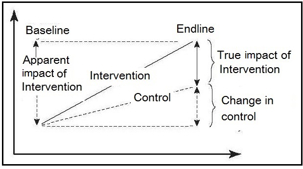
A probability evaluation, when properly executed, provides the highest level of evidence that the inter­vention caused the outcome, and is considered the gold standard method. The method requires the use of a random­ized, controlled, double-blind experimental design, in which the partic­ipants are randomly assigned to either the inter­vention or the control group. Randomization is conducted to ensure that, within the limits of chance, the treat­ment and control groups will be comparable at the start of the study. In some random­ized trials, the treat­ment groups are communities and not individuals, in which case they are known as “community” trials.

Figure 1.1 illustrates the importance of the partic­ipants being random­ized to either the inter­vention or the control group when the control group outcomes have also improved as a result of nonprogram factors.

Note that the inter­vention and control groups are similar at baseline in this figure as a result of randomization.

1.1.5 assessment systems in a clinical setting

The types of nutritional assessment systems used in the community have been adopted in clinical medicine to assess the nutritional status of hospitalized patients. This practice has arisen because of reports of the high preva­lence of protein-energy malnu­trition among surgical patients in North America and elsewhere (Corish and Kennedy, 2000; Barker et al., 2011). Today, nutritional assessment is often performed on patients with acute traumatic injury, on those undergoing surgery, on chronically ill medical patients, and on elderly patients. Initially, screening can be carried out to identify those patients requiring nutritional management. A more detailed and comprehensive baseline nutritional assessment of the individual may then follow. This assessment will clarify and expand the nutritional diagnosis, and establish the severity of the malnu­trition. Finally, a nutri­tion inter­vention may be implemented, often incorporating nutritional monitoring and an evaluation system, to follow both the response of the patient to the nutritional therapy and its impact. Further details of protocols that have been developed to assess the nutritional status of hospital patients are given in Chapter 27.

Personalized nutri­tion is also a rapidly expanding approach that is being used in a clinical setting, as noted earlier. The approach tailors dietary recom­men­dation to the specific biological requirements of an individual on the basis of their health status and performance goals. The latter are not restricted to the prevention and/or mitigation of chronic disease but often extend to strategies to achieve optimal health and well-being; some examples of these personal goals are depicted in Table 1.1.

Table 1.1. Examples of personal goals in relation to personal nutri­tion. Data from van Ommen et al. (2017).

Goal	Definition
Weight management	Maintaining (or attaining) an ideal body weight and/or body shaping that ties into heart, muscle, brain and metabolic health
Metabolic health	Keeping metabolism healthy today and tomorrow
Cholesterol	Reducing and optimizing the balance between high-density lipoprotein and low-density lipoprotein cholesterol in individuals in whom this is disturbed
Blood pressure	Reducing blood pressure in individuals who have elevated blood pressure
Heart health	Keeping the heart healthy today and tomorrow.
Muscle	Having muscle mass and muscle functional abilities. This is the physio­logical basis or underpinning of the consumer goal of “strength”
Endurance	Sustaining energy to meet the challenges of the day (e.g., energy to do that report at work, energy to play soccer with your children after work)
Strength	Feeling strong within yourself, avoiding muscle fatigue
Memory	Maintaining and attaining an optimal short-term and/or working memory
Attention	Maintaining and attaining optimal focused and sustained attention (i.e., being “in the moment” and able to utilize infor­mation from that “moment”)

Personalized nutri­tion necessitates the use of a systems biology-based approach that considers the most relevant interacting biological mechanisms to formulate the best recom­mendations to meet the well­ness goals of the individual.

1.1.6 Approaches to evaluate the evidence from nutritional assessment studies

In an effort to optimize clinical care, evidence-based medicine (EBM) started as a movement in the early 1990s to enhance clinician's under­standing, critical thinking, and use of the published research literature, while at the same time considering the patient’s values and preferences. It focused on the quality of evidence and risk of bias asso­ciated with the types of scientific studies used in nutritional assessment as shown in the EBM hierachy of evidence pyramid in Figure 1.2, with random­ized controlled trials (RCTs) providing the strongest evidence and hence occupying the top tier.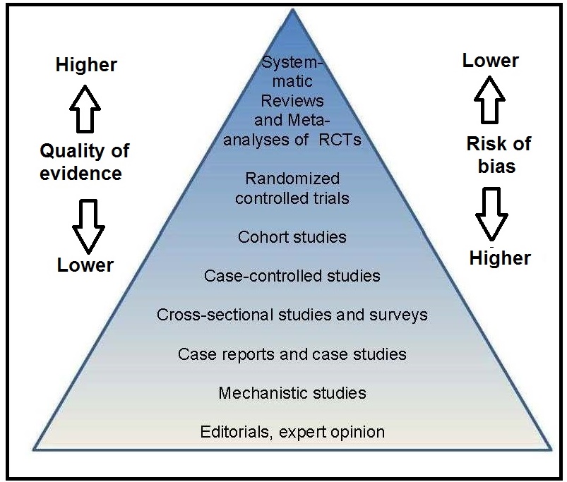

Even within each level there are differences in the quality of evidence, depending on specific design features and conduct of the study. For example, seven bias domains are possible during the course of a study; these are shown in Figure 1.3.

Of these bias domains, the four (i.e., numbers 4–7) that occur after the inter­vention has been assigned can operate in both random­ized and non­randomized study designs, whereas the other three (i.e., numbers 1–3) occur in obser­vational studies and not in well-designed RCTs. Moreover, each bias specified in Figure 1.3 may contain several other different biases; see Hulley et al. (2013) and Yetley et al. (2017a) for more details.

Recognition of the importance of evaluating the evidence from individual studies has led to the development of three tools: Quality Assurance Instruments (QAIs), risk of bias tools, and an evidence-grading system. SIGN 50 is an example of a QAI that is widely used with versions avail­able for cohort studies, case-control studies, and RCTs, and is based on a method­ological checklist of items. In the future, QAIs will be avail­able for nutri­tion studies based on RCTs, cohort, case-control, and cross-sectional studies with the aim of improving the consistency with which nutri­tion studies are assessed.

Risk of bias tools assess the degree of bias and are specific to study type. They focus on internal validity. Examples include the Cochrane Risk of Bias Tool used to evaluate RCTs (Cochrane Handbook), and the (ROBINS-I tool), best used to evaluate individual observational studies (Sterne et al., 2016). These tools assess six of the seven domains of bias listed in Figure 1.3, judging each as low, unclear, or high risk. A nutri­tion-specific risk of bias tool is in the planning stage.

Evidence-grading systems have also been developed for individual studies, of which the Grading of Recom­mendations, assessment, Development and Evaluation (GRADE) approach is widely used (Guyatt et al., 2011), Figure 1.4.

Recognition of the limitations of the initial traditional EBM hierarchy of evidence led to the concept of a system­atic review, now widely used to inform nutri­tion decisions. A system­atic review is the application of scientific strategies to produce comprehensive and repro­ducible summaries of the relevant scientific literature through the system­atic assembly, critical appraisal, and synthesis of all relevant studies on a specific topic (Yetley et al., 2017a). Systematic reviews aim to reduce bias and random error, and provide clarification of the strength and nature of all of the evidence in terms of the quality of research studies, the consistency of the effect, and the evidence of causality. These attributes are particularly useful when there is controversy or conflicting results across the studies (Yetley et al., 2017a).

There are five steps in a system­atic review; these are itemized in Box 1.3. Some of their advantages and disadvantages are summarized in Yetley et al. (2017a)

Systematic reviews that address nutri­tion questions present some unique challenges. Approaches that can be used to address some of these challenges are summarized in Table 1.2

Table 1.2 Applying systemmatic reviews to nutri­tion questions: approaches to the challenges. Data from Brannon (2014).

Challenge	Approach
Baseline exposure	Unlike drug exposure, most persons have some level of dietary exposure to the nutrient or dietary substance of interest, either from food or supplements, or by endogenous synthesis in the case of vitamin D, infor­mation on background intakes and the methodologies used to assess them should be captured in the SR so that any related uncertainties can be factored into data inter­pretation.
Nutrient status	The nutrient status of an individual or popu­lation can affect the response to nutrient supplementation.
Chemical form of the nutrient or dietary substance	If nutrients occur in multiple forms, the forms may differ in their biological activity. Assuring bioequivalence or making use of conversion factors can be critical for appro­priate data inter­pretation.
Factors that influence bioavailability	Depending upon the nutrient or dietary substance, influences such as nutrient-nutrient interactions, drug or food interactions, adiposity, or physio­logical state such as pregnancy may affect the utilization of the nutrient. Capturing such infor­mation allows these influences to be factored into conclusions about the data.
Multiple and interrelated biological functions of a nutrient or dietary substance	Biological functions need to be understood in order to ensure focus and to define clearly the nutrient- or dietary substance—specific scope of the review.
Nature of nutrient or dietary substance inter­vention	Food-based inter­ventions require detailed documentation of the approaches taken to assess nutrient or dietary substance intake.
Uncertainties in assessing dose- response relation­ships	Specific documentation of measure­ment and assay procedures is required to account for differences in health outcomes.

The outcome of a system­atic review is an evidence-based review (EBR) which may include quantitative processes such as meta-analyses to analyze and synthesize the data across the studies. However, combining the results of individual studies can lead to misleading conclusions unless the tools described above are applied to ensure the inclusion of the candidate studies is appro­priate and they are of high quality. Tools are also avail­able for assessing the overall quality of the evidence generated from a system­atic review and meta-analyses. Examples are AMSTAR 2007 and AMSTAR 2 which are avail­able for the conduct , reporting, and subsequent meta-analyses of system­atic reviews based on RCTs and non-random­ized studies, respectively. For details see AMSTAR. In addition, several Web-based collaborative system­atic review tools are avail­able (e.g., SRDR).

Risk of bias tools are also avail­able for system­atic reviews, depending on whether the studies included are random­ized or non-random­ized. Examples include ROBINS for RCTs and ROBIS that can assess risk of bias in both random­ized and nonrandomized studies.

Evidence-grading systems (Figure 1.4) are also used in system­atic reviews. Many use GRADE (Guyatt et al., 2011) which uses evidence summaries to systematically grade the evidence as high, moderate, low, or very low for a series of outcomes.

For all system­atic reviews, it is important to separate the tasks, with a system­atic review team that is separate from the expert group responsible for reviewing the evidence and interpreting the results. Some examples of the misuse of meta-analysis which has led to misleading conclusions can be found in Barnard et al. (2017). Guidelines and guidance to avoid some of the limitations highlighted are avail­able in Dekkers et al. (2019).

Through the Guideline Development Groups (GDGs) at WHO, system­atic reviews are now used to inform the scientific judgment needed for sound evidence-based public health nutri­tion. The process is used to establish nutrient reference values (NRVs), food-based dietary guidelines, and clinical or public health practice guidelines in dietetics and nutri­tion.

1.2 Nutritional assessment methods

Historically, nutritional assessment systems have focused on methods to characterize each stage in the development of a nutritional deficiency state. The methods were based on a series of dietary, labora­tory-based bio­markers, anthro­pometric, and clinical observations used either alone or, more effectively, in combination.

Today, these same methods are used in nutritional assessment systems for a wide range of clinical and public health applications. For example, many low and middle-income countries are now impacted by a triple burden of malnu­trition, where under­nutri­tion, multiple micro­nutrient deficiencies, and over­nutrition co-exist. Hence, nutritional assessment systems are now applied to define multiple levels of nutrient status and not just the level asso­ciated with a nutrient deficiency state. Such levels may be asso­ciated with the maintenance of health, or with reduction in the risk of chronic disease; sometimes, levels leading to specific health hazards or toxic effects are also defined (Combs, 1996).

There is now increasing emphasis on the use of new functional tests to determine these multiple levels of nutrient status. Examples include functional tests that measure immune function, muscle strength, glucose metabolism, nerve function, work capacity, oxidative stress, and genomic stability (Lukaski and Penland, 1996; Mayne, 2003; Russell, 2015; Fenech, 2003).

The correct inter­pretation of the results of nutritional assessment methods requires consid­eration of other factors in addition to diet and nutri­tion. These may often include socio­economic status, cultural practices, and health and vital statistics, which collectively are sometimes termed “ecological factors”; see Section 1.2.5. When assessing the risk of acquiring a chronic disease, environmental and genetic factors are also important (Yetley et al., 2017a).

1.2.1 Dietary methods

Dietary assessment methods provide data used to describe exposure to food and nutrient intakes as well as information on food behaviors and eating patterns that cannot be obtained by any other method. The data obtained have multiple uses for supporting health and preventing disease. For example, health profes­sionals use dietary data for dietary counseling and education and for designing healthy diets for hospitals, schools, long-term care facilities and prisons. At the popu­lation level, national food con­sump­tion surveys can generate infor­mation on nutrient adequacy within a country, identify popu­lation groups at risk, and develop nutri­tion inter­vention programs. Dietary data can also be used by researchers to study relation­ships between diet and disease, and for formulating nutri­tion policy such as food-based dietary guidelines (Murphy et al., 2016).

It is important to recognize that nutrient inadequacies may arise from a primary deficiency (low levels in the diet) or because of a secondary deficiency. In the latter case, dietary intakes may appear to meet nutritional needs, but conditioning factors (such as certain drugs, dietary components, or disease states) interfere with the ingestion, absorption, transport, utilization, or excretion of the nutrient(s).

Several dietary methods are avail­able, the choice depending primarily on both the study objec­tives and the character­istics of the study group (see Chapter 3 for more details). Recently, many technical improvements have been developed to improve the accuracy of dietary methods. These include the use of digital photographs of food portions displayed on a cell-phone or a computer tablet, or image-based methods utilizing video cameras, some wearable. Some of these methods rely on active image capture by users, and others on passive image capture whereby pictures are taken automatically. Under development are wearable camera devices which objectively measure diet without relying on user-reported food intake (Boushy et al., 2017). Several on-line dietary assessment tools are also avail­able, all of which standardize interview protocols and data entry: they can be interviewer‑ or self‑administered (Cade, 2017); see Chapter 3 for more details.

Readers are advised to consult Intake — a Center for Dietary assessment that provides technical assistance for the planning, collection, analysis and use of dietary data. Examples of their avail­able publications are presented in Box 1.4. In addition, recommendations for collecting, analyzing, and interpreting dietary data to inform dietary guidance and public health policy are also avail­able; see Murphy et al., (2016) and Subar et al., (2015) for more details. Data on knowledge, attitudes and practices, and reported food‑related behaviors are also collected. Historically, this has involved observing the participants, as well as in‑depth interviews and focus groups — approaches based on ethnological and anthropological techniques. Today, e‑health (based on the internet) and m‑health (based on mobile phones) communication technologies are also being used to collect these data, as noted earlier (Olson, 2016). All these methods are particularly useful when designing and evaluating nutri­tion inter­ventions.

Often, infor­mation on the proportion of the popu­lation “at risk” of inadequate intakes of nutrients is required. Such infor­mation can be used to ascertain whether assessment using more invasive methods based on nutritional bio­markers are warranted in a specific popu­lation or subgroup.

1.2.2 Laboratory Methods

Laboratory methods are used to measure nutritional biomarkers which are used to describe status, function, risk of disease, and response to treat­ment. They can also be used to describe exposure to certain foods or nutrients, when they are termed “dietary biomarkers”. Most useful are nutritional bio­markers that distinguish deficiency, adequacy and toxicity, and which assess aspects of physio­logical function and/or current or future health. However, it must be recognized that a nutritional bio­marker may not be equally useful across different applications or life-stage groups where the critical function of the nutrient or the risk of disease may be different (Yetley et al., 2017b).

The Bio­markers of Nutrition and Development (BOND) program (Raiten and Combs, 2015) has defined a nutritional bio­marker as:

“a biological characteristic that can be objectively measured and evaluated as an indicator of normal biological or pathogenic processes, and/or as an indicator of responses to nutri­tion inter­ventions”.

Nutritional bio­markers can be measure­ments based on biological tissues and fluids, on physio­logical or behavioral functions and, more recently, on metabolic and genetic data that in turn influence health, well-being, and risk of disease. Yetley and colleagues (2017b) have highlighted the difference between risk bio­markers and surrogate bio­markers. A risk bio­marker is defined by the Institute of Medicine (2010) as a bio­marker that indicates a component of an individual’s level of risk of developing a disease or level of risk of developing complications of a disease. As an example, metabolomics is being used to investigate potential risk bio­markers of pre-diabetes that are distinct from the known diabetes risk indicators (glycosylated hemoglobin levels, fasting glucose, and insulin) (Wang-Sattler et al., 2012).

BOND classified nutritional bio­markers into three groups shown in Box 1.5, based on the assumption that an intake-response relationship exists between the bio­markers of exposure (i.e., nutrient intake) and the bio­markers of status and function. Functional physio­logical and behavioral bio­markers are more directly related to health status and disease than are the functional biochem­ical bio­markers shown in Box 1.5. Disturbances in these functional physiological and behavioral bio­markers are generally asso­ciated with more prolonged and severe nutrient deficiency states, and are often affected by social and environmental factors so their sensitivity and specificity are low. In general, functional physio­logical tests (with the exception of physical growth) are not suitable for large-scale nutri­tion surveys: they are often too invasive, they may require elaborate equip­ment, and the results tend to be difficult to interpret because of the lack of cutoff points. Details of functional physio­logical or behavioral tests dependent on specific nutrients are summarized in Chapters 16–25.

The growing preva­lence of chronic diseases has led to investigations to identify bio­markers that can be used as substitutes for chronic disease outcomes (Yetley et al., 2017b). Chronic disease events are characterized by long developmental times, and are multifactorial in nature with challenges in differen­tiating between casual and associative relations (Yetley et al., 2017b). To qualify as a bio­marker that is intended to substitute for a clinical endpoint, the bio­marker must be on the major causal pathway between an inter­vention (e.g., diet or dietary component) and the outcome of interest (e.g., chronic disease). Such bio­markers are termed “surrogate” bio­markers; only a few such bio­markers have been identified for chronic disease. Examples of well accepted surrogate bio­markers are blood pressure within the pathway of sodium intake and cardiovascular disease (CVD) and low density lipoprotein-cholesterol (LDL) concen­tration within a saturated fat and CVD pathway; see Yetley et al (2017b) for more details.

Increasingly, it is recognized that a single bio­marker may not reflect exclusively the nutritional status of that single nutrient, but instead be reflective of several nutrients, their interactions, and metabolism. This has led to the development of “all‑in‑one” instrument platforms that conduct multiple micro­nutrient tests in a single sample aliquot, as noted earlier. A 7‑plex micro­array immunoassay has been developed for ferritin, soluble transferrin receptor, retinol binding protein, thyroglobulin, malarial antigenemia and inflam­mation status bio­markers (Brindle et al., 2019), which has subsequently been applied to dried blood spot matrices (Brindle et al., 2019). Comparisons with reference‑type assays indicate that with some improvements in accuracy and precision, these multiplex instrument platforms could be useful tools for assessing multiple micro­nutrient bio­markers in national micro­nutrient surveys in low resource settings (Esmaeili et al., 2019). Readers are advised to consult the Micronutrient Survey Manual and Toolkit developed by the U.S. Centers for Disease Control and Prevention (CDC) for details on planning, implementation, analysis, reporting, dissemination and the use of data generated from a national cross-sectional micronutrient survey. For details, see (CDC, 2020).

1.2.3 Anthro­pometric methods

Anthro­pometric methods involve measure­ments of the physical dimensions and gross compo­sition of the body (WHO, 1995). The measure­ments vary with age (and sometimes with sex and race) and degree of nutri­tion, and they are particularly useful in circum­stances where chronic imbalances of protein and energy are likely to have occurred. Such disturbances modify the patterns of physical growth and the relative proportions of body tissues such as fat, muscle, and total body water.

In some cases, anthro­pometric measure­ments can detect moderate and severe degrees of malnu­trition, but cannot identify specific nutrient deficiency states. The measure­ments provide infor­mation on past nutritional history, which cannot be obtained with equal confidence using other assessment techniques.

Anthro­pometry is used in both clinical and public health settings to identify the increasing burden of both under- and over-nutri­tion that now co-exist, especially in low‑ and middle-income countries. Measure­ments can be performed relatively quickly, easily, and reliably using portable equip­ment, provided standardized methods and calibrated equip­ment are used (Chapters 10 and 11). To aid in their inter­pretation, the raw measure­ments are generally expressed as an index, such as height-for-age (See Section 1.3).

Standardized methods exist to evaluate anthro­pometric indices based on Z‑scores or percen­tiles, both calculated in relation to the distri­bution of the corresponding anthro­pometric index for the healthy reference popu­lation (Section 1.5.1 and Section 1.5.2). Often Z‑scores of below −2 or above +2 are used to designate individuals with either unusually low or unusually high anthro­pometric indices, especially in low income countries. When used in this way, the combination of index and reference limit is termed an “indicator”, a term that relates to their use in nutritional assessment, often for public health, or social/medical decision-making (see Chapter 13 for more details).

There is growing concern about the global pandemic of obesity; individuals with obesity are at higher risk of several chronic diseases, including coronary heart disease, diabetes, and hyper­tension. Consequently, numerous investigators have compared the usefulness of anthro­pometric variables such as body mass index (weight,kg) / (height, m)² (BMI) and waist circum­ference as surrogate measures of obesity. In a meta-analysis of studies with at least a 12mos follow-up, Seo et al. (2017) concluded that waist circum­ference was a better predictor for diabetes than BMI (> 30) in women than men and for all ages > 60y, whereas neither BMI > 30, nor waist circum­ference > 102cm (for men), > 88cm (for women) were significant predictors of hyper­tension.

1.2.4 Clinical methods

A medical history and a physical examination are the clinical methods used to detect signs, (obser­vations made by a qualified examiner) and symptoms (manifestations reported by the patient) asso­ciated with malnu­trition or risk of chronic disease. The latter is defined by IOM (2010) as a culmination of a series of pathogenic processes in response to internal or external stimuli over time that results in a clinical diagnosis­/ailment and health outcomes; examples include diabetes, cancer, coronary heart disease, stroke, and arthritis. The signs and symptoms may be nonspecific and develop only during the advanced stages of a nutrient deficiency (or excess) or chronic disease; for this reason, their diagnosis should not rely exclusively on clinical methods. It is obviously desirable to have the capacity to detect marginal nutrient deficiencies and risk of chronic disease before a clinical syndrome develops.

Several labora­tory-based bio­markers exist to assess an individual’s level of risk of developing a disease and as substitutes for chronic disease outcomes; they are often included as an adjunct to clinical assessment. Examples include serum ferritin for risk of iron deficiency anemia, glycosylated hemo­globin (HbA1c) for risk of diabetes, and alterations in bone mineral density for changes in fracture risk. Examples of surrogate bio­markers intended to substitute for chronic disease outcomes include LDL cholesterol instead of the true clinical outcome CVD and blood pressure for cardiovascular disease, as noted earlier (Yetley et al., 2017b).

1.2.5 Ecological factors

Increasingly, nutritional assessment methods include the collection of infor­mation on a variety of other factors known to influence the nutritional status of individuals or populations. This increase has stemmed, in part, from the the United Nations Children’s Fund (UNICEF) conceptual framework for the causes of childhood malnu­trition shown in Figure 1.5, and the increasing focus on studies of diet and chronic disease (Yetley et al., 2017a).

The UNICEF framework highlights that child malnu­trition is the outcome of a complex causal process involving not just the immediate deter­minants such as inadequate dietary intake and poor care, but also the under­lying and basic enabling deter­minants depicted in Figure 1.5.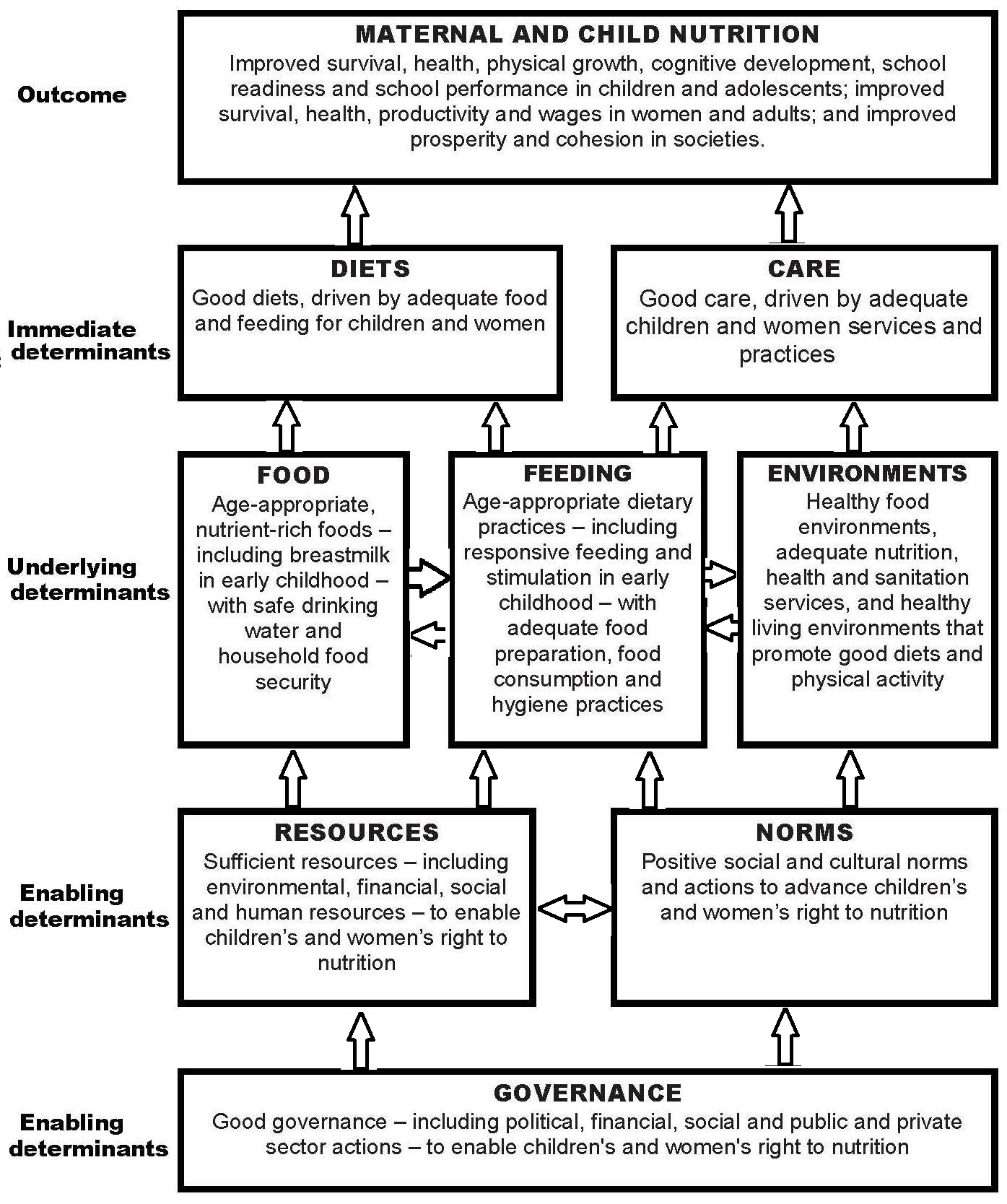

As a consequence, several variables asso­ciated with the under­lying and enabling deter­minants of child malnu­trition are included in nutritional assessment systems, including in the Demographic Health Surveys conducted in low‑ and middle-income countries. Variables addressing the under­lying deter­minants include house­hold compo­sition, education, literacy, ethnicity, religion, income, employment, women’s empower­ment, material resources, water supply, house­hold sanitation, and hygiene (i.e, WASH) and access to health and agricultural services, as well as land ownership and other infor­mation.

Additional data on food prices, the adequacy of food preparation equip­ment, the degree of food reserves, cash-earning oppor­tunities, and the percentage of the house­hold income spent on certain foods such as animal foods, fruits, and vegetables can also be collected, if appro­priate.

Data on health and vital statistics may also be obtained, as may infor­mation on the percentage of the popu­lation with ready access to a good source of drinking water, the proportion of children immunized against measles, the proportion of infants born with a low birth weight, the percentage of mothers practicing exclusive breastfeeding up to six months, and and age‑ and cause-specific mortality rates.

Some of these non-nutritional variables are strongly related to malnu­trition and can be used to identify at‑risk individuals during surveillance studies. For example, Morley (1973) identified birth order over seven, breakdown of marriage, death of either parent, and episodes of infectious diseases in early life as being important factors in the prediction of West African children who were nutritionally at risk. In a study in the state of Maharashtra in India, Aguayo et al. (2016) reported that after controlling for potential confounding, the most consistent predictors of stunting and poor linear growth in children under 23mos were birth­weight and child feeding, women’s nutri­tion and status, and house­hold sanitation and poverty. Women’s empower­ment has also been shown to significantly influence child nutri­tion, infant and young child feeding practices, and reproductive health service utilization in some studies (Kabir et al., 2020).

1.3 Nutritional assessment indices and indicators

Raw measure­ments alone have no meaning unless they are related to, for example, the age or sex of an individual (WHO, 1995). Hence, raw measure­ments derived from each of the four methods are often (but not always) combined to form “indices.” Examples of such combinations include height-for-age, nutrient density (nutrient intake per megajoule), BMI ((weight kg) / (height m)²), and mean cell volume ((hematocrit) / (red blood cell count)). These indices are all continuous variables. Construction of indices is a necessary step for the inter­pretation and grouping of measure­ments collected by nutritional assessment systems, as noted earlier.

Indices are often evaluated in clinical and public health settings by comparison with pre­deter­mined reference limits or cutoff points (Section 1.5). Reference limits in anthro­pometry in low income countries are often defined by Z‑scores below −2, as noted earlier. For example, children aged 6–60mos with a height-for-age Z‑score < −2 are referred to as “stunted”. When used in this way, the index (height‑for‑age) and the asso­ciated reference limit (i.e., < −2 Z‑score) are together termed an “indicator”, a term used in nutritional assessment, often for public health or social/medical decision-making at the popu­lation level.

Several anthro­pometric indicators have been recom­mended by the WHO. For example, they define “underweight” as a weight-for-age < −2 Z‑score, “stunted” as length/height-for-age < −2 Z‑score), and “wasted” as weight-for-length/height < −2 Z‑score. In children aged 0–5y, WHO uses a Z‑score above +2 for BMI‑for‑age as an indicator of “overweight”, and above +3 as an indicator of obesity (de Onis and Lobstein, 2010). Anthro­pometric indicators are frequently combined with dietary and micro­nutrient bio­marker indicators for use in public health programs to identify populations at risk; some examples are presented in Table 1.3.

Table 1.3. Examples of dietary, anthro­pometric, labora­tory, and clinical indicators and their application. EAR, estimated average requirement; IDD, iodine deficiency disorders.

Nutritional indicator	Application
Dietary indicators
Prevalence of the popu­lation with zinc intakes below the estimated average requirement (EAR)	Risk of zinc deficiency in a popu­lation
Proportion of children 6–23mos of age who receive foods from 4 or more food groups	Prevalence of minimum dietary diversity
Anthro­pometric indicators
Proportion of children age 6–60mos in the popu­lation with mid-upper arm circum­ference < 115mm	Risk of severe acute malnu­trition in the popu­lation
Percentage of children < 5y with length- or height-for-age less than −2.0 SD below the age-specific median of the reference popu­lation	Risk of zinc deficiency in the popu­lation
Lab. indicators based on micronutrient biomarkers
Percentage of popu­lation with serum Zn concen­trations below the age/sex/time of day-specific lower cutoff	Risk of zinc deficiency in the popu­lation
Percentage of children age 6–71mos in the popu­lation with a serum retinol < 0.70µmol/L	Risk of vitamin A deficiency in the popu­lation
Median urinary iodine <20µg/L based on > 300 casual urine samples	Risk of severe IDD in the popu­lation
Proportion of children (of defined age and sex) with two or more abnormal iron indices (serum ferritin, erythrocyte protoporphyrin, transferrin receptor) plus an abnormal hemoglobin	Risk of iron deficiency anemia in the popu­lation
Clinical indicators
Prevalence of goiter in school-age children ≥ 30%	Severe risk of IDD among the children in the popu­lation
Prevalence of maternal night blindness ≥ 5%	Vitamin A deficiency is a severe public health problem

Indicators should be chosen carefully in relation to both the study objec­tives and their attributes. They can be used to meet a variety of objec­tives. For example, if the objec­tive of the program is to evaluate the treat­ment of malnu­trition, then the indicator chosen must have the potential to respond to the specific inter­vention under study and must relate to the nature and severity of the malnu­trition present. Thus, the same indicators are not appro­priate for evaluating the treat­ment of stunting versus wasting. Further, several factors will affect the magnitude of the expected response of an indicator. These may include the degree of deficiency, age, sex, and physio­logical state of the target group. Other influencing factors may be the type and duration of the inter­vention, home diet, the age‑specificity of the response, and whether the indicator is homeo­statically controlled. A more detailed discussion of the selec­tion criteria for indicators can be found in Habicht et al. (1980), Habicht and Pelletier (1990), and Habicht and Stoltzfus (1997).

1.4 The design of nutritional assessment systems

The design of the nutritional assessment system is critical if time and resources are to be used effectively. The assessment system used, the type and number of measure­ments selected, and the indices and indicators derived from these measure­ments will depend on a variety of factors.

Efforts have increased dramatically in the past decade to improve the content and quality of nutritional assessment systems, especially those involving clinical trials. In 2013, guidelines were published on clinical trial protocols entitled: Standard Protocol Items: Recommendations for International Trials (SPIRIT). This has led to the compulsory pre­regis­tration of clinical trials, and often publication of the trial protocols in scientific journals. The SPIRIT checklist consists of 33 recom­mended items to include in a clinical trial. Chan et al. (2013) provide the rationale, a detailed description, and model example of each item. Discussions on compulsory pre­regis­tration of protocols for observational studies are in progress; see Lash and Vandenbroucke (2012).

An additional suggestion to support transparency and reproducibility in clinical trials, and to distinguish data-driven analyses from pre-planned analyses is the publication of a statistical analysis plan before data have been accessed (DeMets et al., 2017; Gamble et al., 2017). Initially, recommendations for a pre-planned statistical analyses plan were compiled only for clinical trials (Gamble et al., 2017), but have since been modified for observational studies by Hiemstra et al. (2019) to include details on the adjustment for possible confounders. Tables of the recom­mended content of statistical analysis plans for both clinical trials and observational studies are also avail­able in Hiemstra et al. (2019).

1.4.1 Study objec­tives and ethical issues

The general design of the assessment system, the raw measure­ments, and, in turn, the indices and indicators derived from these measure­ments should be dictated by the study objec­tives. Possible objec­tives may include:

1. Determining the overall nutritional status of a popu­lation or subpopulation
2. Identifying areas, populations, or subpopulations at risk of chronic malnu­trition
3. Characterizing the extent and nature of the malnu­trition within the popu­lation or subpopulation
4. Identifying the possible causes of malnu­trition within the popu­lation or subpopulation
5. Designing appro­priate inter­vention programs for high-risk populations or subpopulations
6. Monitoring the progress of changing nutritional, health, or socio­economic influences, including inter­vention programs
7. Evaluating the efficacy and effectiveness of inter­vention programs
8. Tracking progress toward the attainment of long-range goals.

The first three objec­tives can be met by a cross-sectional nutri­tion survey, often involving all three of the major methods of nutritional assessment. Such surveys, however, are unlikely to provide infor­mation on the possible causes of malnu­trition (i.e., objec­tive no. 4). The latter can only be achieved through interventions (objectives no. 5 and no. 7) and possibly objective no. 6. An assessment of the possible causes of malnu­trition is a necessary prerequisite when implementing nutri­tion inter­vention programs.

In some circum­stances, the objec­tive may be to identify only those individuals at risk of malnu­trition and who require inter­vention (i.e., objec­tive no. 5). To achieve this objec­tive, a screening system is required that uses simple and cheap measure­ments and reflects both past and present nutritional status.

Ethical issues

Formal guidelines on the general conduct of biomedical research is contained in the declaration of Helsinki on Ethics and Epidemiology, published by the Council for International Organization of Medical Sciences (CIOMS, 2016). Ethical approval from the appro­priate human ethics committees in the countries involved in the research study must be obtained by the principal investigators before work begins. The basic guidelines for research on human subjects must be followed. As an example, sections of the regulations of the U.S. Department of Health and Human Services (2021) are shown in Box 1.6. A more detailed discussion of the main ethical issues when planning an application for research ethical approval is avail­able in Gelling (2016).

Informed consent must be obtained from the partic­ipants or their principal caregivers in all studies. When securing informed consent, the investigator should also:

• Disclose details of the nature and procedures of the study
• Clearly state the asso­ciated potential risks and benefits
• Confirm that participation in the research is voluntary
• Confirm that partic­ipants are free to withdraw from the study at any time
• Explain how the results relating to individual partic­ipants will be kept confidential
• Describe the procedures that provide answers to any questions and further infor­mation about the study.

With the increasing reliance on random­ized clinical trials (RCT) to inform evidence-based practice, there have been coordinated attempts to standardize reporting and to register infor­mation about trials for consistency and transparency. This has led to the publication of the Consolidated Standards of Reporting Trials (CONSORT). The CONSORT guidelines specify details that should be well-defined in every RCT, and many journals now require these guidelines to be addressed as a condition of publication. The first CONSORT guidelines were published in 2001 and were revised in 2010 and updated frequently. See: Moher et al. (2012).

In 2004, members of the International Committee of Medical Journal Editors (ICMJE) agreed to require registration of any RCT submitted for review and possible publication (DeAngelis et al., 2004). Several registries have been developed which meet the following ICMJE criteria. These include the registry should be accessible to the public; there should be no charge for registration; open to all interested registrants, managed by a nonprofit organization, and have a means for verifying the validity of the registered infor­mation (Elliot, 2007).

Standards have now been developed to Strengthen Observational Studies in Epidemiology (STROBE). The STROBE guidelines include 18 items common to three study designs, with four additional items specific for cohort, case-control, or cross-sectional studies (von Elm et al., 2014). Registration of protocols for observational studies may be mandatory in the future (Williams et al., 2010).

Standards have also been developed for reporting qualitative research. Two reporting standards are often used — the Consolidated Criteria for Reporting Qualitative Research (COREQ) (32‑item checklist) (Tong et al., 2007) and the Standards for Reporting Qualitative Research (SRQR) (21‑item checklist (O'Brien et al., 2014). Their use can assist researchers to report important aspects of the research team, study methods, context of the study, findings, analysis and inter­pretations.

1.4.2 Choosing the study partic­ipants and the sampling protocol

Nutritional assessment systems often target a large popu­lation — perhaps that of a city, province, or country. That popu­lation is best referred to as the “target popu­lation”. To ensure that the chosen target popu­lation has demographic and clinical character­istics of relevance to the question of interest, a specific set of inclusion criteria should be defined. However, for practical reasons, only a limited number of individuals within the target popu­lation can actually be studied. Hence, these individuals must be chosen carefully to ensure the results can be used to infer infor­mation about the target popu­lation. This can be achieved by defining a set of exclusion criteria to eliminate individuals who it would be unethical or inappro­priate to study; as few exclusion criteria as possible should be specified. The technique of selecting a sample representative of the target popu­lation and of a size adequate for achieving the primary study objec­tives, requires the assistance of a statistician; only a very brief review is provided here.

A major factor influencing the choice of the sampling protocol is the availability of a sampling frame. Additional factors include time, resources, and logistical constraints. The sampling frame is usually a comprehensive list of all the individuals in the popu­lation from which the sample is to be chosen. In some circum­stances, the sampling frame may consist of a list of districts, villages, institutions, school or house­holds, termed “sampling units” rather than individuals per se.

When a sampling frame is not avail­able, nonprobability sampling methods must be used. Three nonprobabilty sampling methods are avail­able: consecutive sampling, convenience sampling, and quota sampling, each of which is described briefly in Box 1.7. Note that the use of nonprobability sampling methods produces samples that may not be representative of the target popu­lation and hence may lead to system­atic bias: such methods should be fully documented. 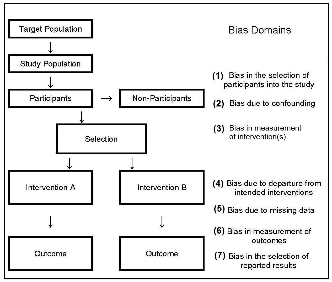Several possible sources of bias can occur when nonprobability sampling is used, as shown by the three domains (nos 1–3) depicted in Figure 1.3. Some specific examples include the following:

• Ignoring people who do not respond to an initial approach to include them in the study — the non-response bias. People who refuse to take part may have character­istics that differ markedly from those of the respondents.
• Studying only volunteers who are often unrepre­sentative of most of the popu­lation.
• Sampling only those persons attending a clinic, school, or health center, and neglecting to include non-attendees.
• Collecting data at only one time of the year, which may introduce a seasonal bias.
• Selecting partic­ipants who are accessible by road introduces a “tarmac” bias. Areas accessible by road are likely to be system­atically different from those that are more difficult to reach.

It is essential to fully document the charac­teristics of the sample and to identify the probable direction and magnitude of the bias that arises from the adopted sample protocol and nonres­ponse rate. Extrapolating the results from a nonprobability sample to the target popu­lation is risky and should be avoided.

Every attempt should be made to compile some type of sampling frame, or to use one that already exists, so that probability sampling can be used (Lemeshow et al., 1990). Probability sampling is the recom­mended method for obtaining a representative sample with minimum bias.

In settings where maps and census data are out of date or non-existent such as in poor urban environments, creating a sampling frame to select a representative sample is particularly challenging. Investigators working in urban slums in four low-income countries have described a method for creating a spatially-referenced sampling frame consisting of a census of all house­holds in a slum from which a spatially-regulated representative sample can be generated; see the Improving Health in Slums Collaborative (2019) for more details.

Several probability sampling methods exist: simple random sampling, system­atic sampling, stratified random sampling, cluster sampling, and multistage sampling. Every effort must be made to minimize the number of nonrespondents so that the generalizability (i.e., external validity) of the study is not compromised. The level of nonres­ponse that will compromise the generalizability of the study depends on the nature of the research question and on the reasons for not responding. Strategies exist for minimizing refusal to participate in the study; see Hulley et al. (2013) for more details.

Of the probability sampling methods, three are described in Box 1.8; further details can be found in Varkevisser et al. (1993).

Cluster sampling requires defining a random sample of natural groupings (clusters) of individuals in the popu­lation. This method is used when the popu­lation is widely spaced and it is difficult to compile a sampling frame, and thus sample from all its elements. Statistical analysis must take clustering into account because cluster sampling tends to result in more homogeneous groups for the variables of interest in the popu­lation.

Stratified sampling results in a sample that is not necessary representative of the actual popu­lation. The imbalance can be corrected, however, by weighting, allowing the results to be generalized to the target popu­lation. Alternatively, a sampling strategy, termed proportional stratification, can be used to adjust the sampling before selecting the sample, provided infor­mation on the size of the sampling units is avail­able. This approach simplifies the data analysis and also ensures that subjects from larger communities have a pro­portion­ately greater chance of being selected than do subjects from smaller communities.

Multistage random sampling is frequently used in national nutri­tion surveys. It typically involves sampling at four stages: at the provincial or similar level (stage one), at the district level (stage two), at the level of communities in each selected district (stage three), and at the house­hold level in each chosen community (stage four). A random sample must be drawn at each stage. The U.S. NHANES III, the U.K. Diet and Nutrition surveys, and the New Zealand and Australian national nutri­tion surveys all used a combination of stratified and multistage random sampling techniques to obtain a sample representative of the civilian non-institutionalized populations of these countries.

As can be seen, each probability sampling protocol involves a random selec­tion procedure to ensure that each sampling unit (often the individual) has an equal probability of being sampled. Random selec­tion can be achieved by using a table of random numbers, a computer program that generates random numbers, or a lottery method; each of these procedures is described in Varkisser et al. (1993).

1.4.3 Calculating sample size

The appro­priate sample size for a particular nutritional assessment project should be estimated early in the process of developing the project design so that, if necessary, modifications to the design can be made. The number of partic­ipants required will depend on the study objec­tive, the nature and scope of the study, and the “effect size” — the magnitude of the expected change or difference sought. The estimate obtained from the sample size calculation represents the planned number of individuals with data at outcome, and not the number who should be enrolled. The investigator should always plan for dropouts and individuals with missing data.

The first step in the process of estimating the sample size is restating the research hypothesis to one that proposes no difference between the groups that are being compared. This restatement is called the “null” hypothesis. Next, the “alternative” hypothesis should be stated, which, if one-sided, specifies the actual magnitude of the expected “effect size” and the direction of the difference between the predictor and outcome variable. In most circum­stances, however, a two-sided alternative hypothesis is stated, in which case only the effect size is specified and not the direction.

The second step in the estimation of sample size is the selec­tion of a reasonable effect size (and variability, if necessary). As noted earlier, this is rarely known, so instead both the effect size and variability must be estimated based on prior studies in the literature, or selected on the basis of the smallest effect size that would be considered clinically meaningful. Sometimes a small pilot study is conducted to estimate the variability (s²) of the variable. When the outcome variable is the change of a continuous measure­ment (e.g., change in a child's length during the study), the s² used should be the variance of this change.

The third step involves setting both α and β. The probability of committing a type 1 error (rejecting the null hypothesis when it is actually true) is defined as α. Another widely used name for α is the level of significance. It is often set at 0.05, when it represents a 95% assurance that a significant result will not be achieved when it should not (i.e., the null hypothesis will not be rejected). If a one-tailed alternative hypothesis has been set, then a one-tailed α should be used; otherwise, use a two-tailed α.

The probability of committing a type II error (i.e.,failing to reject the null hypothesis when it is actually false) is defined as “β”, and is often set at 0.20, indicating that the investigator is willing to accept a 20% chance of missing an association of the specified effect size if it exists. The quantity 1−β is called the power, and when set at 0.80 implies there is a 80% chance of finding an association of that size or greater when it really exists.

The final step involves selecting the appro­priate procedure for estimating the sample size. Two different procedures can be used depending on how the effect size is specified. Frequently, the objec­tive is to determine the sample size to detect differences in the Proportion of individuals in two groups. For example, the proportion of male infants age 9mos who develop anemia while being treated with iron supplements (Hemoglobin < 110g/L) is to be compared to the proportion who develop anemia while taking a placebo. The procedure is two‑sided, allowing for the possibility that the placebo is more effective than the supplement! Note that the effect size is the difference in the projected proportions in the two groups and that the size of that differences critically controls the required sample size. See, Sample size calculator - two proportions.

In a cohort or experimental study, the effect size is the difference between P₁, the proportion of individuals expected to have the outcome in one group and P₂, the proportion expected in the other group. Again, this required effect size must be specified, along with α and β to calculate the required sample size.

In contrast, in a case-control study, P₁ represents the proportion of cases expected to have a particular dichotomous predictor variable (i.e., the preva­lence of that predictor), and P₂ represents the proportion of controls who are expected to have the dichotomous predictor.

For examples when the effect size is specified in terms of relative risk or odds ratio (OR), see Browner et al. in Chapter 6 in Hulley et al. (2013).

Alternatively, the objec­tive may be to calculate an appro­priate sample size to detect if the mean value of a continuous variable in one group differs significantly from the mean of another group. For example, the objec­tive might be to examine the mean HAZ‑score of city childen aged 5y with their rural counterparts aged 5y. The sample size procedure assumes that the distri­bution of the variable in each of the two groups will be approximately normal. However, the method is statistically robust, and can be used in most situations with more than about 40 individuals in each group. Note that in this cases the effect size is the numerical difference in the means of the two groups and that the group variance must also be defined. See, Sample size calculator - two means. However,this sample size calculator cannot be used for studies involving more than two groups, when more sophisticated procedures are needed to determine the sample size.

A practical guide to calculating the sample size is published by WHO (Lwanga and Lemeshow, 1991). The WHO guide provides tables of minimum sample size for various study conditions (e.g., studies involving popu­lation proportion, odds ratio, relative risk, and incidence rate), but the tables are only valid when the sample is selected in a statistically random manner. For each situation in which sample size is to be determined, the infor­mation needed is specified and at least one illustrative example is given. In practice, the final sample size may be constrained by cost and logistical considerations.

1.4.4 Collecting the data

Increasingly, digital tablets rather than paper-based forms are used for data collection. Their use reduces the risk of transcription errors, and can protect data security through encryption. The transport and storage of multiple paper forms is eliminated and costs can be reduced by the elimination of extensive data entry. Several proprietary and open-source software options (e.g., Open Data Kit) are avail­able for data collection. Initially, data are usually collected and stored locally offline, but uploaded on to a secure central data store when internet access is avail­able.

The process of data aquisition, organisation, and storage should be carefully planned in advance, with the objec­tive of facilitating subsequent data handling and analysis and minimising data entry errors — a particular problem with dietary data.

1.4.5 Additional considerations

Of the many additional factors affecting the design of nutritional assessment systems, the acceptability of the method, respondent burden, equip­ment and personnel requirements, and field survey and data processing costs are particularly important. The methods should be acceptable to both the target popu­lation and the staff who are performing the measure­ments. For example, in some settings, drawing venous blood for biochem­ical determinations such as serum retinol may be unacceptable in infants and children, whereas the collection of breast milk samples may be more acceptable. Similarly, collecting blood specimens in populations with a high preva­lence of HIV infections may be perceived to be an unacceptable risk by staff performing the tests.

To reduce the nonres­ponse rate and avoid bias in the sample selec­tion, the respondent burden should be kept to a minimum. In the U.K. Diet and Nutrition Survey, the seven-day weighed food records were replaced by a four-day estimated food diary, when the rolling program was introduced in 2008 due to concerns about respondent burden (Ashwell et al., 2006). Alternative methods for minimizing the nonres­ponse rate includes the offering of material rewards and the provision of incentives such as regular medical checkups, feedback infor­mation, social visits, and telephone follow-up.

The requirements for equip­ment and personnel should also be taken into account when designing a nutritional assessment system. Measure­ments that require elaborate equip­ment and highly trained technical staff may be impractical in a field survey setting; instead, the measure­ments selected should be relatively noninvasive and easy to perform accurately and precisely using rugged equip­ment and unskilled but trained assistants. The ease with which equip­ment can be transported to the field, maintained, and calibrated must also be considered.

The field survey and data processing costs are also important factors. Increasingly, digital tablet devices are being used for data collection in field surveys rather than paper-based forms. As noted earlier, adoption of this method reduces the risk of transcribing error, protects data security through encryption and reduces the cost of extensive data entry. Several proprietary and open-source software options are avail­able, including Open Data Kit, RedCap, and Survey CTO. Software such as Open Data Kit permits offline data collection, automatic encryption, and the ability to upload all submissions when a data collection devise, such as a notebook, is connected to the internet.

In surveillance systems, the resources avail­able may dictate the number of malnour­ished individuals who can subsequently be treated in an inter­vention program. When resources are scarce, the cutoff point for the measure­ment or test (Section 1.5.3) can be lowered, a practice that simultaneously decreases sensitivity, but increases specificity, as shown in Table 1.7. As a result, more truly malnour­ished individuals will be missed while at the same time fewer well-nourished individuals are misdiagnosed as malnour­ished.

1.5 Important characteristics of assessment measures

All assessment measures vary in their validity, sensitivity, specificity, and predictive value; these characteristics, as well as other important attributes, are discussed below,

1.5.1 Validity

Validity is an important concept in the design of nutritional assessment systems. It describes the adequacy with which a measure­ment or indicator reflects what it is intended to measure. Ideally valid measures are free from random and system­atic errors and are both sensitive and specific (Sections 1.5.4; 1.5.5; 1.5.7; 1.5.8).

In dietary assessment, a method that provides a valid reflection of the true “usual nutrient intake” of an individual is often required. Hence, a single weighed food record, although the most accurate dietary assessment method, would not provide a valid assessment of the true “usual nutrient intake” of an individual, but instead provides a measure­ment of the actual intake of an individual over one day. Similarly, if the bio­marker selected reflects “recent” dietary exposure, but the study objec­tive is to assess the total body store of a nutrient, the bio­marker is said to be invalid. In the earlier U.S. NHANES I survey, thiamine and riboflavin were analyzed in casual urine samples because it was not practical to collect 24h urine samples. However, the results were not indicative of body stores of thiamine or riboflavin, and hence were considered invalid; the determination of thiamine and riboflavin in casual urine samples were not included in U.S. NHANES II or U.S. NHANES III (Gunter and McQuillan, 1990).

In some circum­stances, assessment measures only have “internal” validity, indicating that the results are valid only for the particular group of individuals being studied and cannot be generalized to the universe. In contrast, if the results have “external” validity, or generalizability, then the results are valid when applied to individuals not only in the study but in the wider universe as shown in Figure 1.6.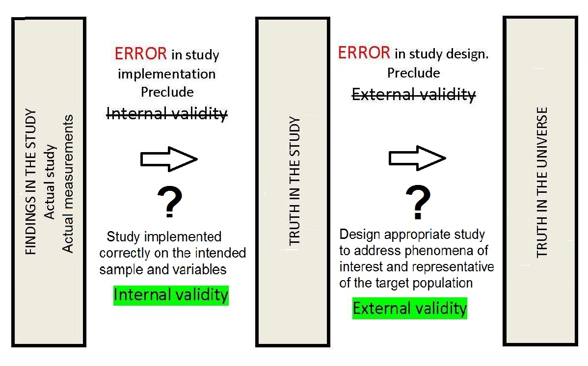

For example, conclusions derived from a study on African Americans may be valid for that particular popu­lation (i.e., have internal validity) but cannot be extrapolated to the wider American popu­lation. Internal validity is easier to achieve. It is necessary for, but does not guarantee, external validity. External validity requires external quality control of the measure­ments and judgment about the degree to which the results of a study can be extrapolated to the wider universe. The design of any nutritional assessment system must include consid­eration of both the internal and external validities of the raw measure­ments, the indices based on them, and any derived indicators, so that the findings can be interpreted accordingly.

1.5.2 Reproducibility or precision

The degree to which repeated measure­ments of the same variable give the same value is a measure of reproducibility — also referred to as “reliability” or “precision” in anthro­pometric (Chapter 9) and laboratory assessment (Chapter 15). The measure­ments can be repeated on the same subject or sample by the same individual (within-observer reproducibility) or different individuals (between-observer reproducibility). Alternatively, the measure­ments can be assessed within or between instruments. Reproducible measure­ments yield greater statistical power at a given sample size to estimate mean values and to test hypotheses.

The study design should always include some replicate observations (repeated but independent measure­ments on the same subject or sample). In this way, the reproducibility of each measure­ment can be calculated. When the measure­ments are continuous, the coefficient of variation (CV%) can be calculated: \[\small \mbox {CV %= standard deviation × 100% / mean}\] For categorical variables, percent agreement, the interclass correlation coefficient, and the kappa statistic can be used.

In anthro­pometry, alternative methods are often used to assess the precision of the measure­ment techniques; these are itemized in Box 1.9, and discussed in Chapter 9. The TEM was calculated for each anthro­pometric measure­ment used in the WHO Multicenter Growth Reference Study for the development of the Child Growth Standards; see de Onis et al. (2004).

The reproducibility of a measure­ment is a function of the random measure­ment errors (Section 1.5.4) and, in certain cases, true variability in the measure­ment that occurs over time. For example, the nutrient intakes of an individual vary over time (within-person variation), and this results in uncertainty in the estimation of usual nutrient intake. This variation characterizes the true “usual intake” of an individual. Unfortunately, within-person variation cannot be distinguished statistically from random measure­ment errors, irrespective of the design of the nutritional assessment system (see Chapter 6 for more details).

The precision of biochem­ical measures is similarly a function of random errors that occur during the actual analytical process and within-person biological variation in the biochem­ical measure. The relative importance of these two sources of uncertainty vary with the different measures. For many modern biochem­ical measures, the within-person biological variation now exceeds the long-term analytical variation, as shown in Table 1.4.

Table 1.4 Within-person and analytical variance components for some common biochem­ical measures. Abstracted from Gallagher et al. (1992).

	Coefficient of variation (%)
Measure­ment	Within-person	Analytical
Serum retinol
Daily	11.3	2.3
Weekly	22.9	2.9
Monthly	25.7	2.8
Serum ascorbic acid
Daily	15.4	0.0
Weekly	29.1	1.9
Monthly	25.8	5.4
Serum albumin
Daily	6.5	3.7
Weekly	11.0	1.9
Monthly	6.9	8.0

A variety of strategies can be used to minimize random measure­ment errors and increase the reproducibility of nutritional assessment systems. These strategies were adopted by the WHO Multicenter Growth Reference Study, and are described in de Onis et al. (2004). They included the following:

• Compiling an operations manual that contains specific written guide­lines for taking each measure­ment, to ensure all the techniques are standardized
• Training all the examiners to use the standardized techniques consistently; the latter is especially important in large surveys involving multiple examiners, and in longi­tudinal studies, where maintaining standardized measure­ment tech­niques during the survey is an important issue
• Carefully selecting and standardizing the instruments used for the data collection; in some cases, variability can be reduced by the use of auto­mated instruments
• Refining and standardizing questionnaires and interview protocols, prefer­ably, where feasible, with the use of computer-administered interview protocols; the latter approach is now often used for 24-h recall interviews in national nutri­tion surveys
• Reducing the effect of random errors from any source by repeating all the measure­ments, when feasible, or at least on a random subsample.

1.5.3 Accuracy

The term “accuracy” is best used in a restricted statistical sense to describe the extent to which the measure­ment is close to the true value. It therefore follows that a measure­ment can be repro­ducible or precise, but, at the same time, inaccurate — a situation which occurs when there is a system­atic bias in the measure­ment (see Figure 1.7 and Section 1.5.5). The greater the system­atic error or bias, the less accurate the measure­ment. Accurate measure­ments, however, necessitate high reproducibility, as shown in Figure 1.7.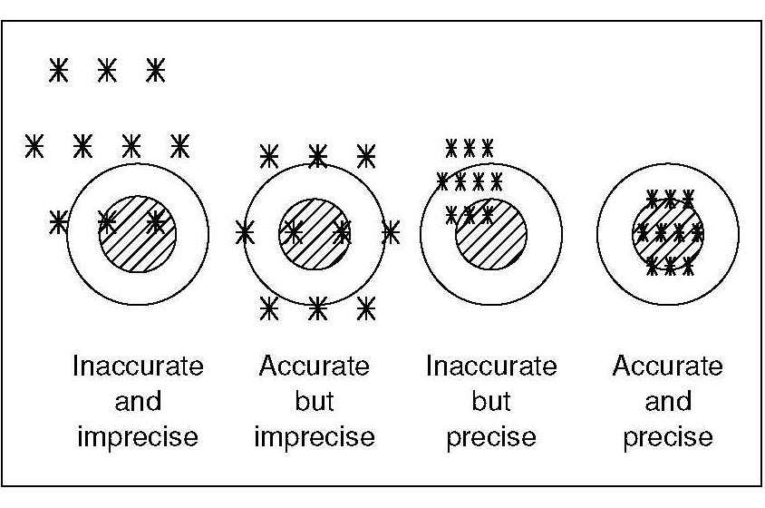

Accuracy is not affected by sample size.

Several approaches exist for assessing the accuracy of a measure­ment, which vary according to the method being used in the nutritional assessment system. Each approach aims to use a reference measure­ment undertaken by a technique that is believed to best represent the true value of the characteristic. The reference method is termed a “gold standard”.

Assessing the accuracy of objec­tive measure­ments of biochem­ical bio­markers is relatively easy and can be accomplished by using reference materials with certified values for the nutrient of interest, prefer­ably with values that span the concen­tration range observed in the study; see Chapter 15 for more details. Certified reference materials can be obtained from the U.S. National Institute of Standards and Technology (e.g., NIST), the U.S. Centers for Disease Control (CDC), the International Atomic Energy Authority (IAEA) in Vienna, the Community Bureau of Reference of the Commission of the European Communities (BCR) in Belgium, and the U.K. National Institute of Biological Standards and Controls (NIBSC).

Table 1.5 Precision and accuracy of measure­ments.

	Precision or reproducibility	Accuracy
Definition	The degree to which repeated measure­ments of the same variable give the same value	The degree to which a measure­ment is close to the true value
Assess by	Comparison among repeated measures	Comparison with certified reference materials, criterion method, or criterion anthropometrist
Value to study	Increases power to detect effects	Increases validity of conclusions
Adversely affected by	Random error contributed by      the measurer,      the respondent, or      the instrument	Systematic error (bias) contributed by:      the measurer,      the respondent, or      the instrument

The control of accuracy in other nutritional assessment methods is more difficult and is discussed in more detail in later chapters. For example, the correct value of any anthro­pometric measure­ment is never known with absolute certainty. In the absence of absolute reference standards, the accuracy of anthro­pometric measure­ments is assessed by comparing them with those made by a designated criterion anthropometrist (Table 1.5). This approach was used in the WHO Multicenter Growth Reference Study; see de Onis et al. (2004) and Chapter 9 for more details.

Accurate measure­ments must also be repro­ducible or precise (Figure 1.7), as noted earlier. Therefore, the same strategies outlined under reproducibility (Section 1.5.2) should be adopted, with the exception of repeating the measure­ments. Additional strategies that can also be used to enhance accuracy include (a) making unobtrusive measure­ments, (b) blinding, and (c) calibrating the instruments. Of these strategies, the first two should always be used to help avoid bias where feasible and appro­priate. An example of a strategy based on unobtrusive measure­ments to enhance accuracy in dietary assessment is surreptitious weighing of food portions consumed by the partic­ipants in institutional settings such as school lunch programs (Warren et al., 2003). Blinding is used in double-blind clinical trials to ensure that neither the partic­ipants nor the researchers know in which group they have been assigned. This strategy, although not ensuring the overall accuracy of the measure­ments, is practiced to minimize the possibility that the apparent effects of the inter­vention are due to differential use of other treat­ments in the inter­vention and control groups, or to biased judgement of the outcome (Hulley et al., 2013). The third strategy, calibrating the instruments, should always be used when any instruments are involved.

The strategies actually adopted to maximize reproducibility and accuracy will depend on several factors. These may include feasibility and cost considerations, the importance of the variable, and the magnitude of the potential impact of the anticipated degree of inaccuracy on the study conclusions (Hulley et al., 2013).

1.5.4 Random errors

Random errors generate a deviation from the correct result due to chance alone. They lead to measure­ments that are imprecise in an unpredictable way, resulting in less certain conclusions. They reduce the precision of a measure­ment by increasing the variability about the mean. They do not influence the mean or median value.

There are three main sources of random error:

• Individual biological variation
• Sampling error
• Measure­ment error

Individual biological variation may be a major source of error (see Table 1.4). Variability due to time of day may affect both anthro­pometric measure­ments (e.g., height) and biochem­ical measure­ments (e.g., serum iron and serum zinc). Some nutritional bio­markers also fluctuate in response to medication or meal con­sump­tion; for serum zinc, for example, variations in response to meal con­sump­tion can be as much as 20% (King et al., 2018).

Sampling may also be a major source of random error. For example, significant sampling errors may be asso­ciated with the selec­tion of respondents, who for practical reasons, are usually a small subset of a larger popu­lation, or with the collection of a particular type of food (e.g., maize porridge) for nutrient analysis. Such errors will be present even if the sampling is truly random. One way to reduce this error is to increase the sample size (i.e., the number of subjects or the number of maize porridge samples).

Measure­ments may also generate random errors. During 24-hr dietary recall interviews, for example, a major source of random measure­ment error may be asso­ciated with the measure­ment of the actual portion size of the foods consumed (Chapter 5). Random measure­ment errors in anthro­pometry may also arise from variations during the measure­ment in the compressibility of the skin by skinfold calipers (Ward and Anderson, 1993) and restless infants when measuring recumbent length.

Random measure­ment errors can be minimized by using standardized measure­ment techniques and trained personnel and by employing rigorous analytical quality-control procedures during labora­tory analysis. However, such errors can never be entirely eliminated. To be sure, random measure­ment errors may be generated when the same examiner repeats the measure­ments (within- or intra-examiner error), or when several different examiners repeat the same measure­ment (between- or inter-examiner error). Details of the quality control procedures that can be incorporated to minimize sources of measure­ment error during dietary and bio­marker assessment are included in Chapter 5 and 15, respectively.

1.5.5 Systematic errors or bias

Unfortunately, system­atic errors may arise in any nutritional assessment method, causing it to become biased. Bias may be defined as a condition that causes a result to depart from the true value in a consistent direction. The errors arising from bias reduce the accuracy of a measure­ment by altering the mean or median value. They have no effect on the variance and hence do not alter the reproducibility or precision of the measure­ment (Himes, 1987).

Several types of bias exist, as shown in Figure 1.3. A detailed list of sources of bias that can affect nutri­tion studies is avail­able in Yetley et al. (2017a), but the principal biases are selec­tion bias and measure­ment bias. All types of nutritional assessment systems may experience selec­tion bias. It arises when there is a system­atic difference between the character­istics of the individuals selected for the study and the character­istics of those who are not, making it impossible to generalize the results to the target popu­lation. Selec­tion bias may originate in a variety of ways. Some of these are outlined in Box 1.10. Wherever possible, a strategy should be used to obtain infor­mation on people who refuse to participate or subsequently fail to complete the study. This infor­mation can then be used to assess whether those who did not participate or dropped out of the study are similar to the partic­ipants. If they differ, then a selec­tion bias is present.

Measure­ment bias can be introduced in a variety of ways. For example:

Biased equip­ment may over- or under­estimate weight or height. Alternatively, skinfold calipers may systematically over- or under-estimate skinfold thickness because of differences in the degree of compression arising from the magnitude of the jaw pressure.

Analytical bias may result from the use of a biochem­ical method that systematically under- or overestimates the nutrient content of a food or biological specimen. For example, vitamin C may be under­estimated because only the reduced form of vitamin C, and not total vitamin C, is measured. Alternatively, if the biopsy specimens of the treat­ment and control groups are analyzed in different laboratories which produce systematically different results for the same assay, then the assay results will be biased.

Social desirability bias occurs, for example, when respondents under­estimate their alcohol con­sump­tion in a 24h food recall or record. However, scales can be used to measure the extent of the bias (Robinson et al., 1991), including the Marlowe-Crowne Social Desirability Scale (Crowne and Marlowe, 1960).

Interviewer bias arises when interviewers differ in the way in which they obtain, record, process, and interpret infor­mation. This is a particular problem if different interviewers are assigned different segments of the popu­lation, such as different racial or age groups.

Recall bias is a form of measure­ment bias of critical importance in retrospective case control studies. In such studies, there may be differential recall of infor­mation by cases and controls. For example, persons with heart disease will be more likely to recall past exposure to saturated fat than the controls, as saturated fat is widely known to be asso­ciated with heart disease. Such a recall bias may exaggerate the degree of effect of association with the exposure or, alternatively, may under­estimate the association if the cases are more likely than controls to deny past exposure.

Bias is important as it cannot be removed by subsequent statistical analysis. Consequently, care must be taken to reduce and, if possible, eliminate all sources of bias in the nutritional assessment system by the choice of an appro­priate design and careful attention to the equip­ment and methods selected. Strategies for controlling bias and its potential effect on the measure­ment of a cause-effect relationship are described in most standard epidemio­logical texts; see Hulley et al. (2013) for more details. For examples of criteria that can be applied to assess the risk of bias depending on the type of study (i.e., RCT, cohort, case-control, cross-sectional), see Yetley et al. (2017a).

1.5.6 Confounding

Confounding is a special type of bias that can affect the validity of a study: it masks the true effect. A confounding variable is defined as a characteristic or variable that is associated with the problem and with a possible cause of the problem. See Howards (2018a; and 2018b). Such a characteristic or variable may either strengthen or weaken the apparent relationship between the problem and possible cause. Three conditions must exist for confounding to occur. These are:

• Confounding factor must be associated with both the risk factor of interest and the outcome;
• Confounding factor must be distributed unequally among the groups being compared;
• A confounder cannot be an intermediary step in the causal pathway from the exposure of interest to the outcome of interest.

Examples of confounders in epidemio­logical studies often include age, gender, and social class. In the example shown in Figure 1.8, cigarette smoking confounds the apparent relationship between coffee con­sump­tion and coronary heart disease and is thus said to be the confounding variable. The latter arises because persons who consume coffee are more likely to smoke than people who do not drink coffee, and cigarette smoking is known to be a cause of coronary heart disease (Beaglehole et al., 1993), (Figure 1.8).

Some authors have drawn a distinction between confounders and other variables that may also influence outcome. The latter include outcome modifiers and effect modifiers. Outcome modifiers have an effect on the health outcome independent of the exposure of interest.

Effect modifiers, in contrast, modify (positively or negatively) the effect of the hypothesized causal variables. Hence, unlike confounders and outcome modifiers, effect modifiers do lie on the causal pathway relating the exposure of interest to the outcome. As an example, hyper­tension is more frequent among African Americans than among Caucasians, whereas the preva­lence of coronary heart disease is higher among Caucasians than among African Americans. Hence, some variable possibly related to lifestyle or constitution may modify the effect of hyper­tension on coronary heart disease. The number of participants needed to study effect modification is generally large, and as a consequence many studies are not powered to detect effect modification. For more details, see Newman et al. in Hulley et al. (2013) Chapter 9.

Several strategies exist to control for confounders, provided they are known and measured. They can be applied at the design or at the analysis stage, although confounding by unmeasured factors may still remain. In large studies, it is preferable to control for confounding at the analysis stage.

Strategies at the design stage include randomization to minimize the influence of baseline confounding variables, and blinding to control a biased judgement of the outcome (for RCTs only) (Section 1.5.5). Alternatively, for observational studies, restriction and matching can be used, also at the design stage; both involve changes in the sampling to ensure that only groups with similar levels of the confounders are compared.

Restriction, the simplest strategy, involves designing inclusion criteria that specify a value for the potential confounding variable, and exclude everyone with a different value. In the example depicted in Figure 1.8, if restriction was applied to avoid confounding, only nonsmokers would be included in the study design so that any association between coffee and heart disease could not be due to smoking. However, such a restriction would compromise the ability to generalize the findings to smokers, and sometimes may adversely affect recruitment, and thus the final sample size.

Matching is another strategy commonly used to control for confounding. It involves selecting individually cases and controls with the same matching values of the confounding variable(s). Both pair-wise matching and matching in groups (i.e., frequency matching) can be used. Unlike restriction, because partic­ipants at all levels of the confounder are studied, generalizability is not compromised in matching. In the Figure 1.8, when applying a case-control design, each case (i.e., person with heart disease) would be individually matched to one or more controls who smoked about the same number of cigarettes per day (i.e., pair-wise matching). The coffee drinking of each case would then be compared with that of the matched control. In some circum­stances confounding variables can be controlled in the design phase without measuring them; these are termed “oppor­tunistic obser­vational designs”. For details, see Hulley et al. (2013)

Alternatively, when controlling for confounders at the analysis stage, potential confounders are not prespecified. Three strategies are avail­able: stratification; statistical modeling; and propensity scores. For stratification, subjects are segregated into strata according to the level of a potential confounder, after which the relation between the predictor and outcome in each stratum are examined separately. Stratification is often limited by the size of the study, and the limited number of covariates that can be controlled simultaneously. In such cases, statistical modeling (multi­variate) can be used to control multiple confounders simultaneously; a range of statistical techniques are avail­able.

Propensity scores are used in observational studies to estimate the effect of a treat­ment on an outcome when selec­tion bias due to nonrandom treat­ment assignment is likely. By creating a propensity score, the goal is to balance covariates between individuals who did and did not receive a treat­ment, making it easier to isolate the effect of a treat­ment; see Garrido et al. (2014). For more details of the advantages and disadvantages of strategies for coping with confounders at both the design and analysis stage, the reader is referred to Nørgaard et al. (2017). For guidelines on the appro­priate use of each of these strategies, consult a statistician.

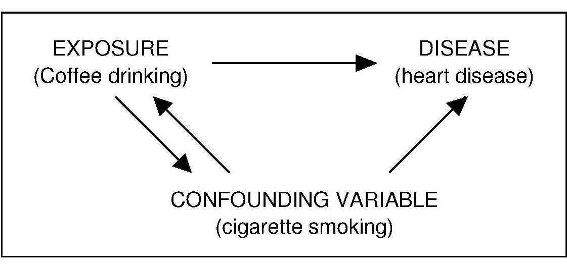
1.5.7 Sensitivity

The sensitivity of a test or indicator refers to the extent to which it reflects nutritional status or predicts changes in nutriture. Sensitive tests (or indicators) show large changes as a result of only small changes in nutritional status. As a result, they have the ability to identify and classify those persons within a popu­lation who are genuinely malnour­ished.

Some variables are strictly homeo­statically controlled, and hence have very poor sensitivity. An example is shown in Figure 1.9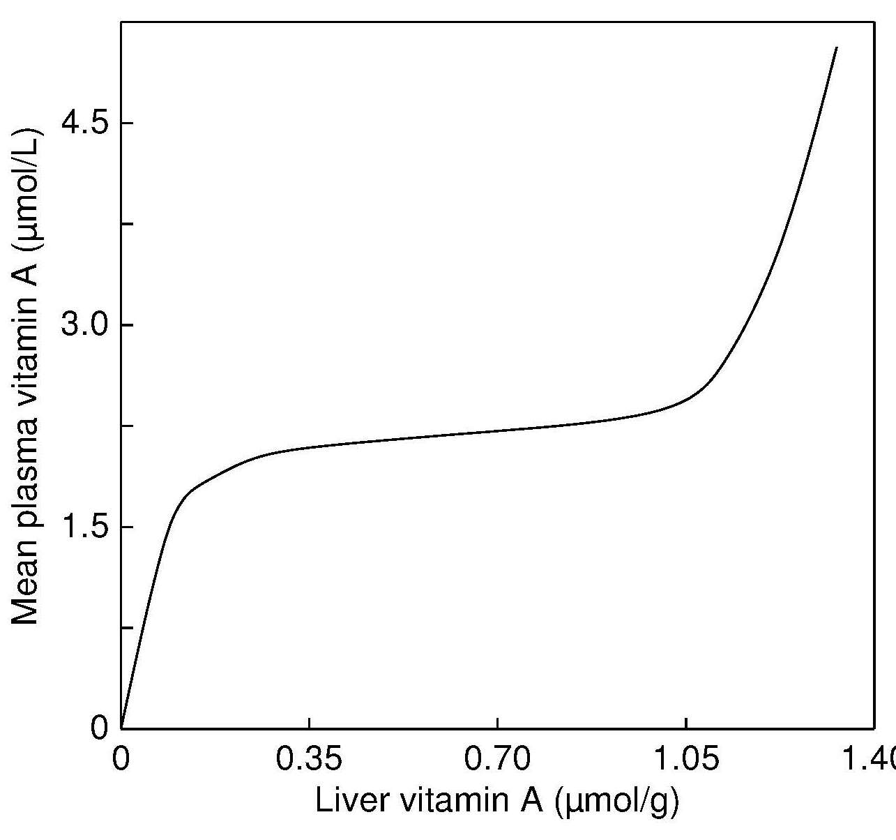

that displays the hypothetical relationship between mean plasma vitamin A and liver vitamin A concen­trations. Note that plasma retinol concen­trations reflect the vitamin A status only when liver vitamin A stores are severely depleted (< 0.07µmol/g liver) or excessively high (> 1.05µmol/g liver). When liver vitamin A concen­trations are within these limits, plasma retinol concen­trations are homeo­statically controlled and levels remain relatively constant and do not reflect total body reserves of vitamin A. Therefore, in populations from higher income countries where liver vitamin A concen­trations are generally within these limits, the usefulness of plasma retinol as a sensitive bio­marker of vitamin A exposure and status is limited.

Likewise, the use of serum zinc as a bio­marker of exposure or status at the individual level is limited due to tight homeostatic control mechanisms. For example, doubling the intake of zinc increases plasma zinc concen­trations by only 6% according to a recent meta-analysis (King, 2018).

An index (or indicator) with 100% sensitivity correctly identifies all those individuals who are genuinely malnour­ished: no malnour­ished persons are classified as “well” (i.e., there are no false negatives). Numerically, sensitivity (S_e) the proportion of individuals with malnu­trition who have positive tests (true positives divided by the sum of true positives and false negatives). The sensitivity of a test (or indicator) changes with preva­lence, as well as with the cutoff point, as discussed in Section 1.6.3.

Unfortunately, the term “sensitivity” is also used to describe the ability of an analytical method to detect the substance of interest. The term “analytical sensitivity” should be used in this latter context (Chapter 15).

1.5.8 Specificity

The specificity of a test (or indicator) refers to the ability of the test (or indicator) to identify and classify those persons who are genuinely well nourished. If a measure­ment (or indicator) has 100% specificity, all genuinely well-nourished individuals will be correctly identified: no well-nourished individuals will be classified as “ill” (i.e., there are no false positives). Numerically, specificity (S_p) is the proportion of individuals without malnu­trition who have negative tests (true negatives divided by the sum of true negatives and false positives).

Table 1.6

Table 1.6: Numerical definitions of sensitivity, specificity, predictive value, and preva­lence for a single index used to assess malnu­trition in a sample group.
    Sensitivity (S_e) = TP / (TP+FN)
    Specificity (S_p) = TN / (FP+TN)
    Predictive value (V) = (TP+TN) / (TP+FP+TN+FN)
    Positive predictive value (V+) = TP / (TP+FP)
    Negative predictive value (V−) = TN / (TN+FN)
    Prevalence (P) = (TP+FN) / (TP+FP+TN+FN)
From Habicht (1980).

Test result	The true situation: Malnutrition present	The true situation:   No malnu­trition
Positive	True positive (TP)	False positive (FP)
Negative	False negative (FN)	True negative (TN)

describes the four situations that are possible when evaluating the performance of a test or indicator. These are a true positive (TP) result: the test is positive and the person really has, for example, anemia; a false-positive (FP) result: the test is positive but the person does not, for example, have anemia; a false-negative (FN) result: the test is negative but the person genuinely has anemia: and a true-negative (TN) result: the test is negative and the person does not have anemia. Increasingly in nutritional assessment, the performance of tests, and their asso­ciated indicators are being evaluated by calculating sensitivity and specificity, as well as predictive value (Section 1.5.10).

It is important to note that sensitivity and specificity only provide infor­mation on the proportion or percentage of persons with or without malnu­trition who are correctly categorized. These measures do not predict the actual number of persons who will be categorized as malnour­ished. The actual number of persons will depend on the frequency of malnu­trition in the group being studied.

The ideal test has a low number of both false positives (high specificity) and false negatives (high sensitivity), and hence the test is able to completely separate those who genuinely are malnour­ished from persons who are healthy. In practice, a balance has to be struck between specificity and sensitivity, depending on the consequences of identifying false negatives and false positives. For example, for a serious condition such as screening for neonatal phenylketonuria, it might be preferable to have high sensitivity and to accept the increased cost of a high number of false positives (reduced specificity). In such circum­stances, follow-up would be required to identify the true positives and true negatives.

Factors modifying sensitivity and specificity

Cutoff points have an effect on both sensitivity and specificity. In cases where lower values of the measure are asso­ciated with malnu­trition (e.g., hemoglobin), decreasing the cutoff point decreases sensitivity but increases specificity for a given test. Conversely, increasing the cutoff will increase sensitivity but decrease specificity. Table 1.7 illustrates this inverse relation between sensitivity and specificity.

Table 1.7. Sensitivity, specificity, and relative risk of death asso­ciated with various values for mid-upper-arm circum­ference in children 6–36mos in rural Bangladesh. Data from Briend et al. (1987).

Arm circum- ference (mm)	Sensitivity (%)	Specificity (%)	Relative Risk of death
≤ 100	42	99	48
100–110	56	94	20
110–120	77	77	11
120–130	90	40	6

Similarly Bozzetti et al. (1985) showed that when the cutoff for total iron binding capacity was lowered from < 310µg/dL to < 270µg/dL, the sensitivity fell from 55% to 30% but the specificity in predicting post­operative sepsis increased from 68% to 87%.

Extent of the random errors asso­ciated with the raw measure­ments influence the specificity and sensitivity of a test. If the asso­ciated random errors are large, the test will be imprecise and both the specificity and sensitivity will be reduced. Although random errors can never be completely eliminated, strategies do exist to minimize them, as noted earlier (Section 1.5.4).

Non-nutritional factors such as inflam­mation, diurnal variation, and the effects of disease may reduce the specificity (Habicht et al.,1979). For example, inflam­mation is known to decrease concen­trations of serum iron, serum retinol, serum retinol binding protein, and serum zinc, while increasing serum ferritin and serum copper (Bresnahan and Tanumihardjo, 2014). As a result, the tests yield values which do not reflect true iron, vitamin A or zinc status, so misclassification occurs; individuals are designated “at risk” to low concen­trations of serum iron, retinol, retinol binding protein, and serum zinc, when they are actually unaffected (false positives). In contrast, inflam­mation increases serum ferritin and serum copper, so that in this case individuals may be designated “not at risk” when they are truly affected by the condition (false negatives).

Table 1.8

Table 1.8. Impact of inflam­mation on micro­nutrient bio­markers of Indonesian infants of age 12mos. From Diana et al. (2017).
     * Ferritin < 12µg/L
     ** RBP < 0.83µmol/L
     *** Zinc < 9.9µmol/L

Bio­marker in serum	Geometric mean (95% CI)	Proportion at risk (%)
Ferritin*: No adjustment	14.5µg/L (13.6–17.5)	44.9
Ferritin: Brinda adjustment	8.8µg/L (8.0–9.8)	64.9
Retinol binding protein**: No adjustment	0.98 (µmol/L) (0.94–1.01)	24.3
Retinol binding protein: Brinda adjustment	1.07µmol/L (1.04–1.10)	12.4
Zinc***: No adjustment	11.5µmol/L (11.2–11.7)	13.0
Zinc: Brinda adjustment	11.7µmol/L (11.4–12.0)	10.4

illustrates the impact of inflam­mation on the geometric mean and preva­lence estimates of iron, vitamin A, and zinc deficiency based on serum ferritin, retinol binding protein, and zinc.

A new regression modeling approach has been developed to adjust serum micro­nutrient concen­trations when affected by inflam­mation. In this new approach used in Table 1.8, the inflammatory bio­markers (serum C-reactive protein (CRP) and α‑1‑acid glycoprotein (AGP) are treated as continuous variables allowing the full range and severity of the inflam­mation to be accounted for; see Suchdev et al. (2016) for more details. Other disease processes may also alter the nutrient status, and in turn, the specificity of a test; for examples, see Table 15.5 in Chapter 15 (Bio­markers).

Biological and behavioral processes that relate the indicator to the outcomes may influence sensitivity and specificity. The sensitivity of low birth weight as an indicator of neonatal mortality will be greater in settings where it is due largely to prematurity rather than to intrauterine growth retardation. The sensitivity or specificity of dietary intake data collected during 24hr interviews may be affected by behavioral effects. Participants have admitted in postsurvey focus group interviews to altering their eating patterns; reasons include inconvenience, embarrassment and guilt (Macdiarmid and Blundell, 1997).

1.5.9 Prevalence

The number of persons with malnu­trition or disease during a given time period is measured by the preva­lence. Numerically, the actual preva­lence (P) is the proportion of individuals who really are malnour­ished or infected with the disease in question (the sum of true positives and false negatives) divided by the sample popu­lation (the sum of true positives, false positives, true negatives, and false negatives) (Table 1.6).

Prevalence influences the predictive value of a nutritional index more than any other factor (see Section 1.5.10). For example, when the preva­lence of malnu­trition such as anemia decreases, it becomes less likely that an individual with a positive test (i.e., low hemoglobin) actually has anemia and more likely that the test represents a false positive. Therefore, the lower the preva­lence of the condition, the more specific a test must be to be clinically useful (Hulley et al., 2013).

1.5.10 Predictive value

The predictive value can be defined as the likelihood that a test correctly predicts the presence or absence of malnu­trition or disease. Numerically, the predictive value of a test is the proportion of all tests that are true (the sum of the true positives and true negatives divided by the total number of tests) (Table 1.6). Because it incorporates infor­mation on both the test and the popu­lation being tested, predictive value is a good measure of overall clinical usefulness.

The predictive value can be further subdivided into the positive predictive value and the negative predictive value, as shown in Table 1.6. The positive predictive value of a test is the proportion of positive tests that are true (the true positives divided by the sum of the true positives and false positives). The negative predictive value of a test is the proportion of negative tests that are true (the true negatives divided by the sum of the true negatives and false negatives). In other words, positive predictive value is the probability of the person having malnu­trition or a disease when the test is positive, whereas negative predictive value is the probability of the person not having malnu­trition or disease when the test is negative.

The predictive value of any test is not constant but depends on the sensitivity and specificity of the test, and most importantly, on the preva­lence of malnu­trition or disease in the popu­lation being tested. Table 1.9 shows the influence of preva­lence on the positive predictive value of an index when the sensitivity and specificity are constant. When the preva­lence of malnu­trition is low, even very sensitive and specific tests have a relatively low positive predictive value. Conversely, when the preva­lence of malnu­trition is high, tests with rather low sensitivity and specificity may have a relatively high positive predictive value (Table 1.9).

Table 1.9 Influence of disease preva­lence on the predictive value of a test with sensitivity and specificity of 95%. From Dempsey and Mullen (1987).

Predictive Value	Prevalence 0.1% 1% 10% 20% 30% 40%
Positive	0.02 0.16 0.68 0.83 0.89 0.93
Negative	1.00 1.00 0.99 0.99 0.98 0.97

The predictive value is the best indicator of the usefulness of any test of nutritional status in a particular circumstance. An acceptable predictive value for any test depends on the number of false-negative and false-positive results that are considered tolerable, taking into account the preva­lence of the disease or malnu­trition, its severity, the cost of the test, and, where appro­priate, the availability and advantages of treat­ment. In general, the highest predictive value is achieved when specificity is high, irrespective of sensitivity (Habicht, 1980).

Sometimes, labora­tory measure­ments are combined with measure­ments of nutrient intakes and anthro­pometric measure­ments to form a multiparameter index with an enhanced predictive value. Several examples of multiparameter indices used to identify malnour­ished hospital patients and predict those who are at nutritional risk are discussed in detail in Chapter 27. Of these, the Nutritional Risk Index (NRI), developed by the Veterans Affairs Total Parenteral Nutrition Cooperative Study Group (1988) uses a formula that includes serum albumin level, present weight, and usual weight: \[\small \mbox {NRI = (1.519 × serum albumin)}\] \[\small \mbox {+ 41.7 × (present weight/usual weight ) }\] The NRI was found to be sensitive and specific and a positive predictor for identifying patients at risk for complications in a study of 395 surgical patients (Veterans Affairs TPN Co-operative Study Group, 1991). NRI > 100 indicated not malnour­ished; NRI 97.5–100, mild malnu­trition; NRI 83.5–97.5, moderate malnu­trition; NRI < 83.5, severe malnu­trition.

Increasingly, multiparameter indices based on three nutritional biomarkers of iron status (in combination with CRP and AGP — biomarkers of inflammation) are being used to identify iron deficiency and iron deficiency anemia at the individual and population level. The biomarkers recommended include serum ferritin, soluble transferrin receptor, and hemoglobin (Pfeiffer and Looker, 2017).

1.6 Evaluation of nutritional assessment indices

In popu­lation studies, nutritional assessment indices can be evaluated by comparison with a distri­bution of reference values from a healthy population (if avail­able) using percen­tiles, standard deviation scores (Z‑scores), and in some cases, percent-of-median (See Chapter 13 for more details). Alternatively, for classifying individuals, the values for nutritional assessment indices can be compared with either statistically pre­deter­mined reference limits drawn from the reference distri­bution for a healthy population or cutoff points. The latter are based on data that relate the levels of the indices to low body stores of the nutrient, impaired function, clinical signs of deficiency, morbidity or mortality. Sometimes, more than one reference limit or cutoff point is used to define degrees of malnu­trition (e.g., undernutrition, overweight, obesity with body mass index) (Chapters 9 and 10).

1.6.1 Reference distri­bution

Reference values are obtained from the reference sample group. The distri­bution of these reference values form the reference distri­bution. The relationship between the terms used to define reference values is shown in Box 1.11

Theoretically, only healthy persons are included in the reference sample group. However, few “true” healthy reference distri­butions have been compiled. Exceptions include the distri­butions of growth reference values for the new WHO Child Growth Standards for children aged 0–60mos. These describe the growth of children whose care has followed recom­mended health practices and behaviors asso­ciated with healthy outcomes. Hence, they are said to be prescriptive, depicting physio­logical human growth for children 0–60mos under optimal conditions; for more details see de Onis et al. (2004). The distri­bution of reference values for hemoglobin (by age, sex, and race) compiled from U.S. NHANES III (1988–1991), and for serum zinc (by age, sex, blood collection time/fasting status) compiled from U.S. NHANES 1I (1976-1980), are other examples of a “true” healthy reference distri­butions. They are based on a sample of healthy, nonpregnant individuals, with data from any person with conditions known to affect iron status, or in the second case serum zinc concentrations, excluded (Looker et al., 1997; Hotz et al., 2003). In practice, however, more frequently the reference values for the reference sample group are drawn from the general popu­lation sampled during a nationally representative survey such as U.S. NHANES III (1988–1994) or the U.K. National Diet and Nutrition surveys.

For comparison of the observed values at the individual or population level with data derived from the reference sample, the person(s) under observation should be matched as closely as possible to the reference individuals by the factors known to influence the measure­ment (Ritchie and Palomaki, 2004). Frequently, these factors include age, sex, race, and physio­logical state, and, depending on the variable, they may also include exercise, body posture, and fasting status. In Figure 1.10, the distribution of length/height-for-age scores of male children participating in the Indian National Family Health Survey (2005–2006) are matched by age and sex with the WHO Child Growth Standard for children 0–5y. The time of day used for specimen collection is especially critical for comparison of serum zinc concen­trations with reference data (Hotz et al., 2003). Only if these matching criteria are met can the observed value be correctly interpreted. Figure 1.10

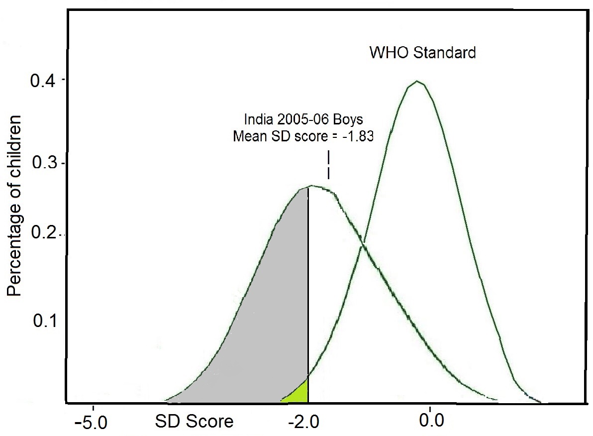
1.6.2 Reference limits

The reference distri­bution can also be used to derive reference limits and a reference interval. Reference limits are generally defined so that a stated fraction of the reference values would be less than or equal to the limit, with a stated probability. Two reference limits may be defined statistically, and the interval between and including them is termed the “reference interval”. Statistically, the reference interval is often the central 95% of a normal reference distri­bution, and is assumed to represent a normal range. Observed values for individuals can then be classified as “unusually low”, “usual”, or “unusually high,” according to whether they are situated below the lower reference limit, between or equal to either of the reference limits, or above the upper reference limit (IFCC,1984).

In low income countries, reference limits for anthro­pometric growth indices based on Z‑scores are preferred, with Z‑scores below −2 or above +2 often used as the reference limits. to designate individuals with either unusually low or unusually high anthropometric indices. When this approach is used, theoretically the proportion of children with a Z‑score less than −2 or greater than +2 in a study population should be about 2.3%. Clearly, if the proportion in the study population with such low or high Z-scores is significantly greater than this, then the study population is seriously affected, as shown in Figure 1.10. The use of Z‑scores is recom­mended in low income countries because Z‑scores can be calculated accurately beyond the limits of the original reference data. In contrast, in industrialized countries, the 3^rd or 5^th and 95^th or 97^th percen­tiles are frequently the reference limits used to designate individuals with unusually low or unusually high anthro­pometric growth indices.

Often for biochem­ical indices, only a lower reference limit is defined. In U.S. NHANES III, the lower reference limit for hemoglobin corresponded to the 5^th percentile of the “true” healthy reference distribution of the U.S. NHANES III (1988–1991) survey, whereas for serum zinc, the lower reference limits (by age, sex, fasting status, and time of blood collection) are based on the 2.5^th percentile values from a “true” healthy reference sample derived from U.S. NHANES II (1976–1980). See Chapter 24 and Hotz et al. (2003).

Note that the terms “abnormal,” or “pathological” should not be applied when using this statistical approach for setting the reference limits because an unusually high or low value for an index is not necessarily asso­ciated with any impairment in health status (Smith et al., 1985).

1.6.3 Cutoff points

Cutoff points, unlike statistically defined reference limits, are based on the relationship between nutritional assessment indices and low body stores, functional impairment, or clinical signs of deficiency or excess, as noted earlier (Raghaven et al. 2016). Their use is less frequent than that of reference limits because infor­mation relating nutritional assessment indices and functional impairment or clinical signs of deficiency or excess is often not avail­able. Figure 1.11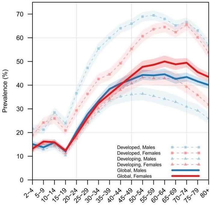

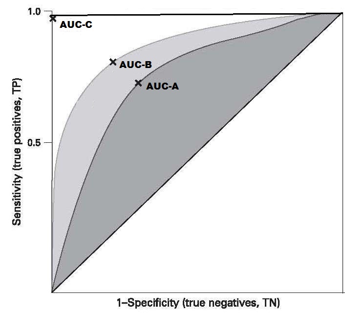
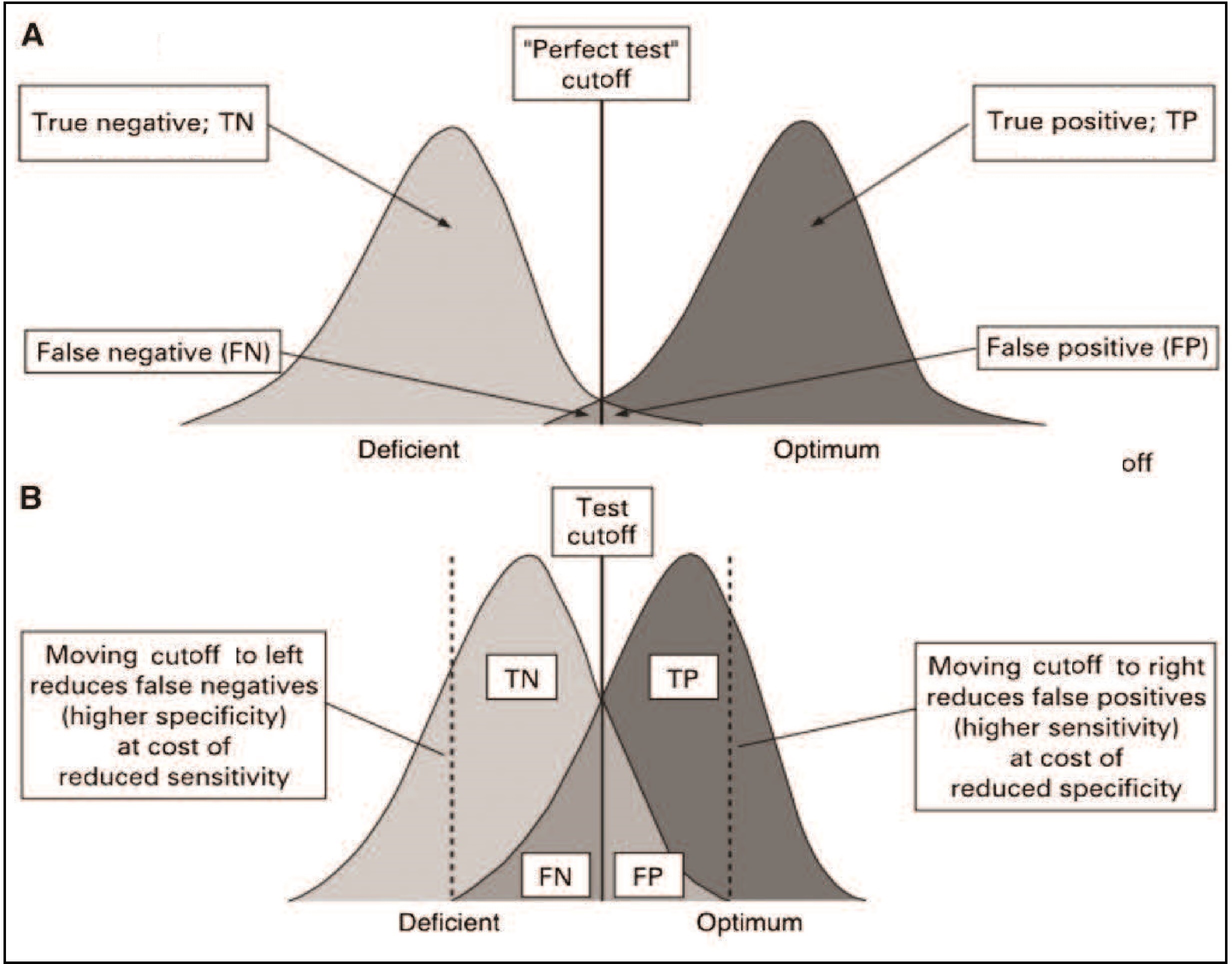
depicts the global prevalence of overweight and obesity for adult males and females based on a population measure (i.e., cutoff for BMI ≥ 25 by age and sex). In this example, a BMI cutoff defined as 25 or higher is based on the evidence that excess weight is associated with an increased incidence of cardiovascular diseases, type 2 diabetes mellitus, hypertension, stroke, dyslipidemia, osteoarthritis, and some cancers (Burton et al., 1985). Cutoff points may vary with the local setting because the relationship between the nutritional indices and functional outcomes is unlikely to be the same from area to area.

Cutoff points, like reference limits, are often age-, race-, or sex-specific, depending on the index. They must also take into account the precision of the measure­ment. Poor precision affects the sensitivity (Section 1.5.7) and specificity (Section 1.5.8) of the measure­ment, and leads to an overlap between those individuals classified as having low or deficient values with those having normal values. This results in misclassification of individuals.

Sometimes more than one cutoff point is selected. For example, several cutoffs based on body mass index (BMI, kg/m²) are used to classify the severity of over­nutrition in adults (see Chapter 10), whereas for serum vitamin B₁₂ two cutoffs asso­ciated with vitamin B₁₂ deficiency or depletion have been defined (Allen et al., 2018). The U.S. Institute of Medicine have published four cutoffs for serum total 25‑hydroxy­vitamin D to define four stages of vitamin D status: deficiency; insufficiency; sufficiency; no added benefit; possible harm (see Chapter 18b for more details), with the limit for deficiency (< 12ng/mL; < 30nmol/L) based on relation­ships to bio­markers of bone health (Ross et al., 2011).

When selecting an index and its asso­ciated cutoff point, the relative importance of the sensitivity and specificity of the nutritional index (or indicator) must always be considered, as noted earlier (Sections 1.5.7, 1.5.8). Receiver operator characteristic (ROC) curves are often used to select cutoff points. This is a graphical method of comparing indices and portraying the trade-offs that occur in the sensitivity and specificity of a test when the cutoffs are altered. To use this approach, a spectrum of cutoffs or thresholds over the observed range of results is required and the sensitivity and specificity for each cutoff calculated. Next, the sensitivity (or true-positive rate) is plotted on the vertical axis against the true negative rate (1.0−specificity) on the horizontal axis for each of the three cutoff points as shown in Figure 1.12.

The closer the curve follows the left-hand border and then the top-border of the ROC space, the more accurate is the bio­marker cutoff in distinguishing a deficiency from optimal status. The optimal ROC curve is the line connecting the points highest and farthest to the left of the upper corner. The closer the curve comes to the 45° diagonal of the ROC space, the less accurate the bio­marker cutoff. Most statistical programs (e.g., SPSS) provide some sort of ROC curve analysis (Søreide, 2009). For more details, see Chapter 15.

The area under the ROC curve (AUC), also known as the cut-point “c” statistic or c index, is a commonly used summary measure of the accuracy of the cutoff for the nutritional assessment index of interest. AUCs can range from 0.5 (random chance, or no predictive ability); this follows the 45° line in the ROC plot, see (Figure 1.10) to > 0.75 (good), and > 0.9 (excellent). The cutoff value that provides the highest sensitivity and specificity is calculated. On the rare occasions that the estimated AUC for the index cutoff is < 0.5, then the index cutoff is worse than chance. When multiple indices are avail­able for the same nutrient, the index with the highest AUC is often selected.

The Youden index (J) is another main summary statistic of the ROC curve. It defines the maximum potential effectiveness of a bio­marker. J can be defined as: \[\small \mbox {J = (maximum sensitivity (c) + specificity (c) − 1}\] The cutoff that achieves the maximum is referred to as the optimal cutoff (c*) because it is the cutoff that optimizes the bio­marker’s differen­tiating ability when equal weight is given to sensitivity and specificity. J can range from 0 to 1, with values closer to 1 indicating a perfect diagnostic test and values closer to 0 signifying a limited effectiveness. For more details, see Schisterman et al. (2005) and Ruopp et al. (2008).

Misclassification arises when there is overlap between individuals who actually have the deficiency (or excess) and those falsely identified (i.e., false positives). Neither reference limits nor cutoff values can separate the “deficient” and the “adequately nourished” without some misclassification occurring. This is shown in Figure 1.13

for the real-life situation (B).

Note that the final selec­tion of the cutoff values may vary depending on whether the consequences of a high number of individuals being classified as false positive is more or less important than the consequences of a large number of individuals being classified as false negatives. Minimizing either misclassification may be considered more important than minimizing the total number of individuals misclassified.

Note that the sensitivity can be improved (i.e., reducing the false positives) by moving the cutoff to the right, but this reduces the specificity (false negatives), whereas moving the cutoff to the left reduces the false negatives (higher specificity) at the cost of a reduction in sensitivity. The former scenario may be preferred for the clinical diagnosis of a fatal condition, whereas cutoffs with a high specificity may be preferred for diagnostic tests that are invasive or expensive.

Misclassification arises because there is always biological variation among individuals (and hence in the physio­logical normal levels defined by the index), depending on their nutrient requirements (Beaton, 1986). As well, for many bio­markers there is high within-person variation, which influences both the sensitivity and specificity of the index, as well as the popu­lation preva­lence estimates. These estimates can be more accurately determined if the effect of within-person variation is taken into account. This can only be done by obtaining repeated measure­ments of the index for each individual, which for invasive biochem­ical bio­markers, is often not feasible .

Figure 1.13 illustrates the problem of misclassification. In this figure, the light-shaded area to the right of 110g/L and below the left curve represents anemic persons classified as normal according to the cutoff point (110g/L) defined by the World Health Organization (WHO, 1972). The dark-shaded area to the left of 110g/L and below the right curve comprises persons within the normal popu­lation, classified as anemic by the WHO cutoff point but who were not found to be responsive to iron administration. Hence, the dark-shaded area represents those well-nourished persons who were incorrectly classified as “anemic” (i.e., false positives).

1.6.4 Trigger levels for surveillance and public health decision making

In popu­lation studies, cutoff points may be combined with trigger levels to set the level of an index (or indicator) or combination of indices at which a public health problem exists of a specified level of concern. Trigger levels may highlight regions or populations, where specific nutrient deficiencies are likely to occur, or may serve to monitor and evaluate inter­vention programs. They should, however, be interpreted with caution because they have not necessarily been validated in popu­lation-based surveys.

Some international organizations including WHO and UNICEF (2018), the International Vitamin A Consultative Group (Sommer and Davidson, 2002), and the International Zinc Nutrition Consultative Group (IZiNCG, 2004), for example, have defined the preva­lence criteria for selected indicators within a popu­lation that signify a public health problem in relation to specific nutrients and conditions.

Table 1.10. Prevalence thresholds, corresponding labels, and the number of countries (n) in different preva­lence threshold categories for wasting, over­weight and stunting in children under 5 years using the “novel approach”. From de Onis et al. (2018).

Wasting			over­weight			Stunting
Prevalence thresholds (%)	Labels	(n)	Prevalence thresholds (%)	Labels	(n)	Prevalence thresholds (%)	Labels	(n)
< 2·5	Very low	36	< 2·5	Very low	18	< 2·5	Very low	4
2·5 – < 5	Low	33	2·5 – < 5	Low	33	2·5 – < 10	Low	26
5 – < 10	Medium	39	5 – < 10	Medium	50	10 – < 20	Medium	30
10 – < 15	High	14	10 – < 15	High	18	20 – < 30	High	30
≥ 15	Very high	10	≥ 15	Very high	9	≥ 30	Very high	44

As an example, the WHO and UNICEF have classified the severity of malnu­trition in young children age < 60mos into five thresholds based on the preva­lence (as %) of wasting (i.e., weight-for-length/height < −2 Z‑scores), overweight (weight-for-age > +2 Z‑scores), and stunting (length/height-for-age < −2 Z‑scores) for targeting purposes (de Onis et al., 2018). The number of countries (i.e. “n”) in each of the different threshold categories, based on data from the WHO 2018 Global Database on Child Growth and Malnutrition, are also shown (Table 1.10).

Comparison of the preva­lence estimates for each anthro­pometric indicator can trigger countries to identify the most appro­priate inter­vention program to achieve “low” or “very low” preva­lence threshold levels. Trigger levels for zinc bio­markers have been set by the Inter­national Zinc Nutrition Consultative Group. (Box 1.12) Note that ideally, all three types of indicators should be used together to obtain the best estimate of the risk of zinc deficiency in a popu­lation and to identify specific sub-groups with elevated risk (de Benoist et al., 2007).

A generalized discussion of the specific procedures used for the evaluation of dietary, anthro­pometric, labora­tory, and clinical methods of nutritional assessment are discussed more fully in Chapters 8, 13, 15, and 25, respectively. CITE AS: Gibson R.S., Principles of Nutritional Assessment: Introduction https://nutritionalassessment.org/
Email: Rosalind.Gibson@Otago.AC.NZ
Licensed under CC-BY-4.0
( PDF ).