Gibson RS1
Principles of
Nutritional Assessment:
Body Composition
3rd Edition, July 2024
Abstract
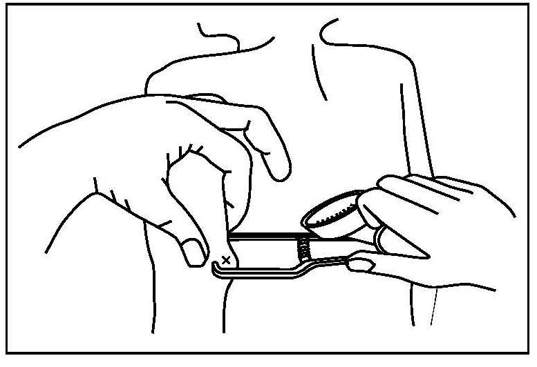
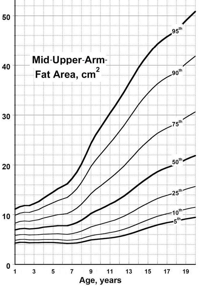
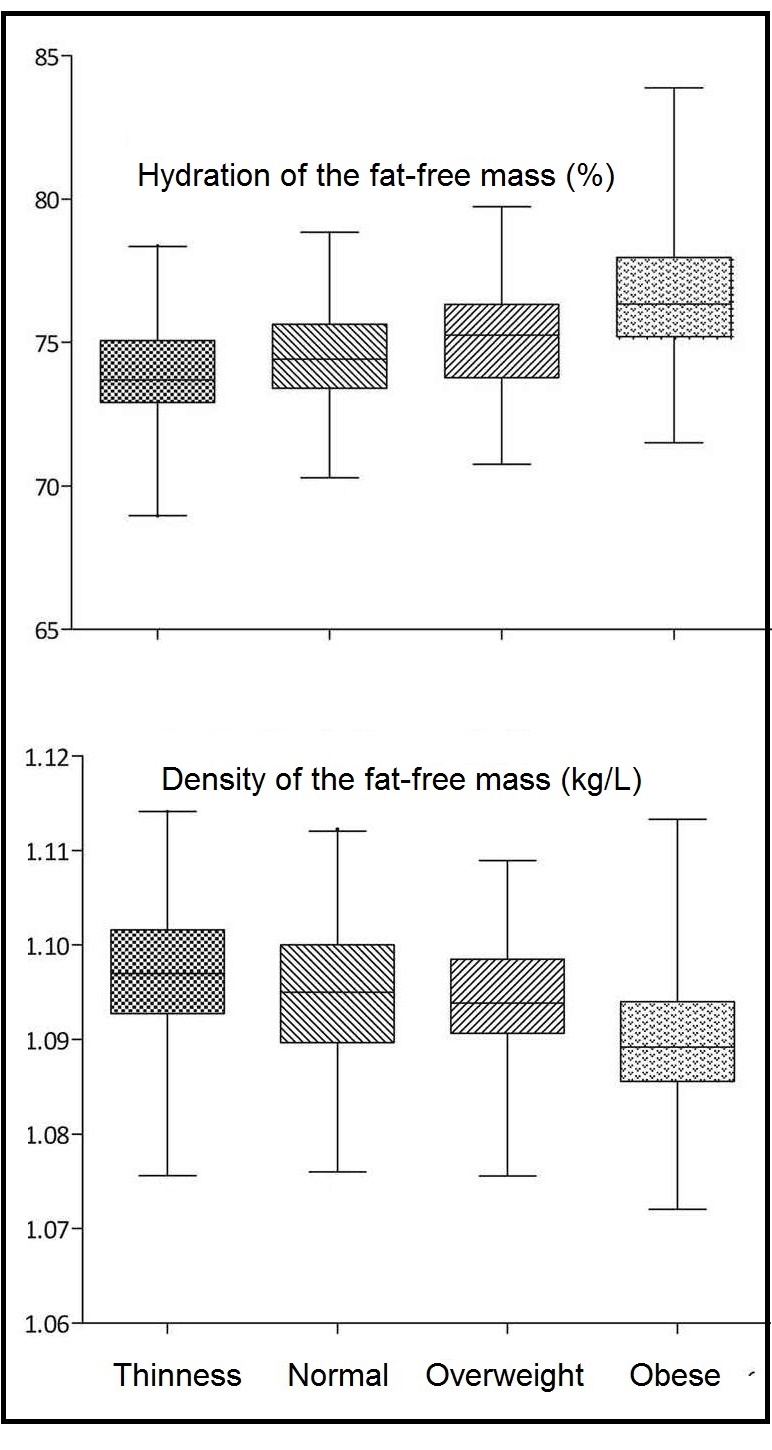
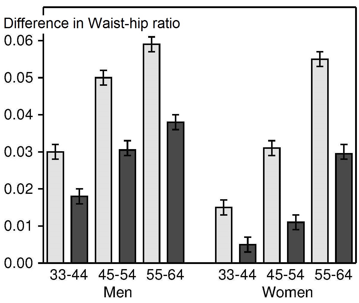
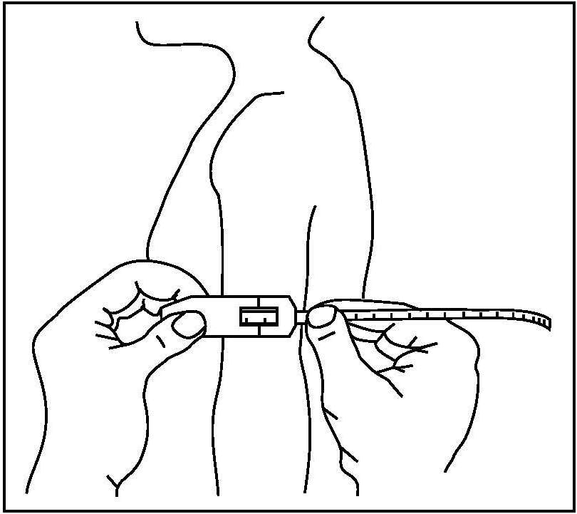
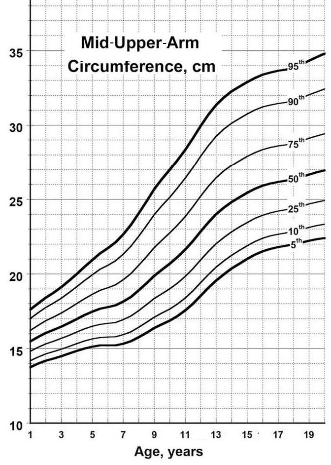
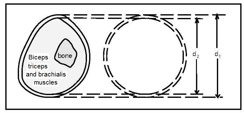
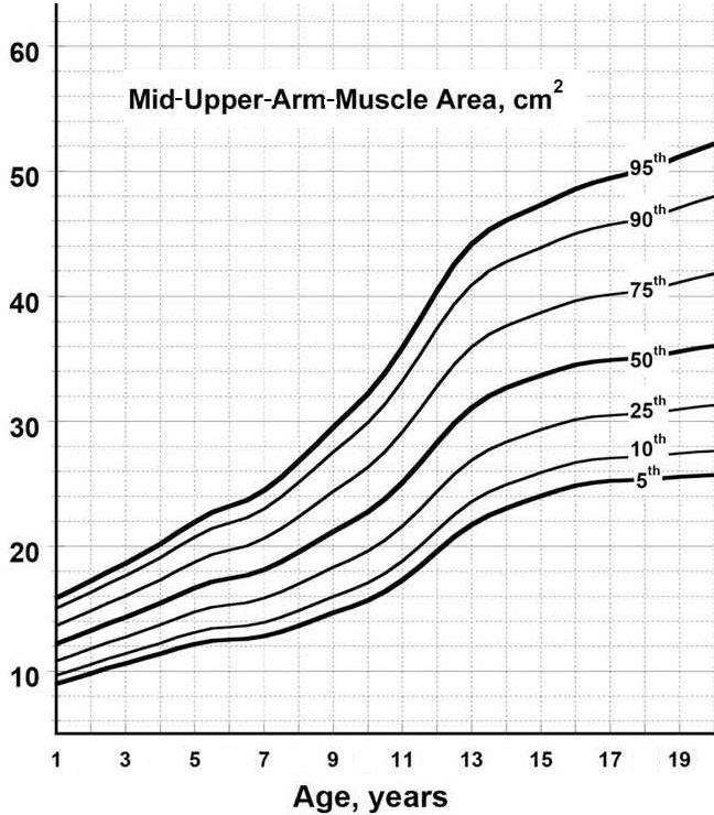
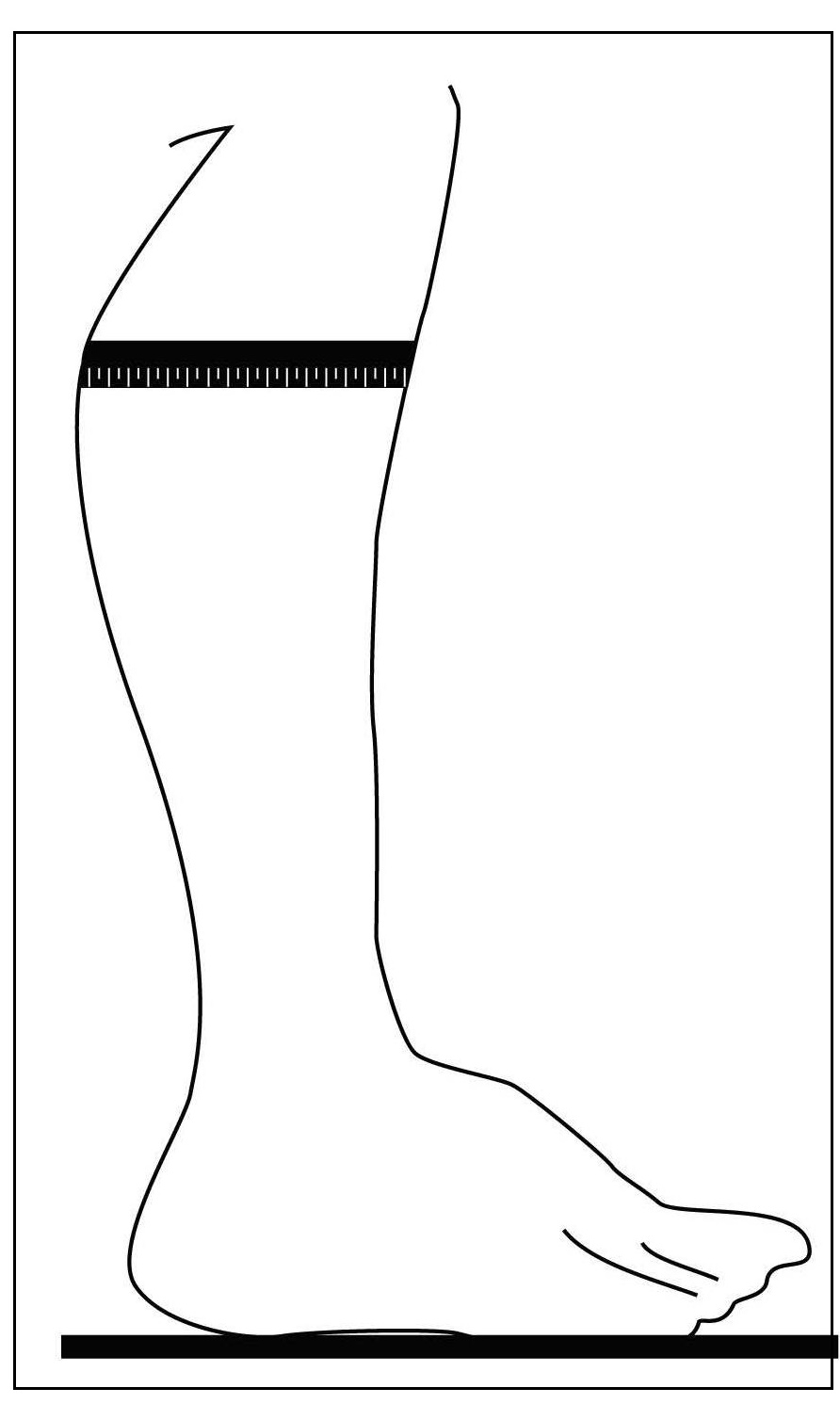
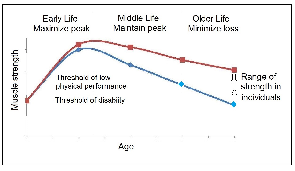
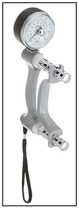
Most anthropometric methods used to assess body composition are based on the two componment model whereby the body consists of fat and fat-free mass. These two body components can be assessed indirectly from selected skinfold thickness and circumference measurements taken by standardized techniques. Several methods exist for estimating percentage body fat and/or total body fat. In the simplest method, skinfold thickness measurements, either singly or in combination, are used to assess body fat (as % or total). Alternatively, percentage body fat can be predicted from adiposity equations matched to the measured skinfolds and study population (by age, gender, ethnicity, activity level, etc). Arm-fat area, calculated from triceps skinfold thickness and mid-upper arm circumference (MUAC), is also used as a proxy for total body fat, although the equation used has some limitations. Both WHO international and population-specific reference data are available for triceps and subscapular skinfolds for children. Arm-fat area data are more limited, although data for U.S. children (1-20y) from the CDC2000 BMI growth chart sample have been compiled. Anthropometric variables from multiple anatomical sites are also used to estimate body density, from which the percentage of body fat, and subsequently, total body fat is calculated. The reliability of this method has been questioned based on comparisons of the derived percentage body fat estimates against those generated using the in vivo gold standard 4-component model which does not rely on any theoretical assumptions. Corrections that account for age, sex, disease state or nutritional status can now be applied to the density-based formulae and/or the empirical equations used to relate fat content to body density, and thus improve the final assessment of body composition. Recognition of the link between the distribution of body fat and risk of cardiovascular disease has prompted use of waist-hip ratio (WHR), and more recently, waist circumference (WC), as practical anthropometric surrogates for intra-abdominal visceral fat. Population-specific cutoffs for adults have been set to denote high WHR or WC indicative of abdominal obesity and cardiovascular risk. Increasingly, WC is being included along with BMI in all obesity surveillance studies. Fat-free mass can be estimated as body weight (kg) minus body fat from the adiposity or density-based methods outlined above. Alternatively, simpler methods include the measurement of MUAC, either alone or combined with triceps skinfold thickness to calculate arm mid-upper-muscle circumference (MUAMC) or arm muscle area (AMA). MUAC alone is used in emergencies to screen for severe acute malnutrition (SAM), whereas MUAMC and AMA can be used as proxies for muscle mass, and thus for the detection of sarcopenia in the elderly. AMA is preferable to MUAMC because it more adequately reflects the true magnitude of tissue changes. Calf circumference and hand grip strength as surrogate markers of skeletal muscle mass and strength respectively, are increasingly being used, in part because loss of both muscle mass and strength has been associated with several adverse health outcomes. Both measurements are recommended by the Asian and European Working Groups on Sarcopenia to identify at risk older adults. The measurements are also used in children and athletes to assess physical fitness. Adiposity has been identified as a confounder of calf circumference measurements, and BMI adjustment factors have been developed. Low calf circumference with any BMI can now be identified. Population-specific calf circumference cutoff values are available to detect low muscle mass in adults. Handgrip strength is said to be a better predictor of functional health outcomes than low muscle mass, and has been linked with alteration in physical performance in cross-sectional studies. Associations with all-cause mortality, cardiovascular mortality, and hospital readmissions have also been observed in prospective cohort studies. Hand grip strength is measured with a calibrated handheld dynamometer. The measurements depend on the model used, but dynamometer-specific cutoffs values are not yet applied. Current cutoffs for weak muscle strength vary across regions; population specific normative reference data are available for the elderly and across the life course. Finally, the cross-sectional nature of the normative reference data compiled for the anthropometric variables discussed limits their use for monitoring the trajectories of individuals and the degree to which causal and age-related inferences can be drawn. None of the anthropometric variables are sensitive enough to monitor small changes in body fat or fat-free mass that may arise after short-term nutritional support or deprivation. CITE AS: Gibson RS. Principles of Nutritional Assessment: Body Composition. https://nutritionalassessment.org/bodycomposition/Email: Rosalind.Gibson@Otago.AC.NZ
Licensed under CC-BY-4.0
( PDF ).