15.1 Biomarkers to assess nutritional status

Nutritional bio­markers are increasingly important with the growing efforts to provide evidence-based clinical guidance, and advice on the role of food and nutrition in supporting health and preventing disease. A nutritional bio­marker has been defined by the Biomarkers of Nutrition and Develop­ment (BOND) program as a biological characteristic that can be objectively measured and evaluated as an indicator of normal biological or patho­genic processes, and/or as an indicator of responses to nutrition inter­ventions (Raiten and Combs, 2015). Thus nutritional bio­markers can be measure­ments based on biological tissues and fluids, on physio­logical or behavioral functions, and more recently, on metabolic and genetic data that in turn influence health, well-being and risk of disease. Most useful are nutritional bio­markers that distinguish deficiency, adequacy and toxicity, and which assess aspects of physio­logical function and/or current or future health. Increasingly, under­standing the effect of diet on health requires the study of mechanisms, not only of nutrients but also of other bioactive food con­stituents at the molecular level. Hence, there is also a need for molecular bio­markers that allow the detection of the onset of disease, in, ideally, the pre-disease state. Unfortunately, nutritional bio­markers are often affected by technical and biological factors other than changes in nutritional status, which can con­found the interpretation of the results.

Nutritional bio­markers are used to support a range of applications at both the population and individual level; these applications are listed below.

At the population level

• National Nutrition surveys: assess overall nutritional status of populations
• Nutrition Screening: identify persons “at risk” in the population via cut-offs
• Surveillance: con­tinuous monitoring of nutritional status of selected population groups over time (e.g., U.S. NHANES and U.K. Diet and Nutrition Survey Rolling Program)
• Monitoring and Evaluation: monitor coverage of / compliance with nutrition policies; evaluate the efficacy and/or effectiveness of public health programs and inter­ventions over time; substantiate health claims.

At the individual level

• In apparently healthy patients: assess reserves, pool size, tissue amounts of the nutrient; determine response to clinical treatment of a nutrient deficiency or disease state
• In “sick” patients: determine status for a specific clinical problem; reflect current status of deficiency or clinical disease; predict future risk of disease or long-term functional outcome if abnormal values persist.

Application list modified from Raiten et al. (2011).

15.1.1 Classification of bio­markers

BOND has classified nutritional bio­markers into three groups, shown in Box 15.1, based on the assumption that an intake-response relationship exists between the bio­marker of exposure (i.e., nutrient intake) and the bio­markers of status and function. Never­the­less, it is recognized that a single bio­marker may not reflect exclusively the nutritional status of that single nutrient, but instead be reflective of several nutrients, their inter­actions, and metabolism. In addition, a nutritional bio­marker may not be equally useful across different applications or life-stage groups where the critical function of the nutrient or the risk of disease may be different.

Biomarkers of exposure are intended to assess what has been con­sumed, and, where possible, take into account bioavail­ability, defined as the proportion of the ingested nutrient that is absorbed and utilized through normal metabolic pathways (Hurrell et al., 2004). Biomarkers of exposure can be based on measure­ments of nutrient intake obtained using traditional dietary assessment methods. Alternatively, depending on the nutrient, nutrient exposure can be measured indirectly, based on surrogate indicators termed “dietary bio­markers”. These are intended to provide a more objective measure of dietary exposure that is independent of the measure­ment of food intake.

Biomarkers of status measure either a nutrient in biological fluids or in tissues, or the urinary excretion rate of the nutrient or its metabolites, often with the aim of assessing where an individual or population stands relative to an accepted cut-off (e.g., adequate, marginal, deficient). Ideally, the bio­marker selected should reflect either the total body con­tent of the nutrient or the size of the tissue store that is most sensitive to depletion. In practice, such bio­markers are not available for many nutrients. Furthermore, even if levels of the nutrient or metabolite in the biological tissue or fluid are “low”, they may not necessarily reflect the presence of a pathological lesion. Alternatively, their significance to health may be unknown.

Biomarkers of function are intended to measure the extent of the functional con­sequences of a specific nutrient deficiency or excess, and hence have greater biological significance than the static bio­markers. Increasingly, functional biomarkers are also being used as substitutes for chronic disease outcomes in studies of associations between diet and chronic disease. When used in this way, they are termed “surrogate biomarkers”; see Yetley et al. (2017) for more details. Functional bio­markers can be subdivided into two groups: functional biochemical, and functional physio­logical or behavioral, bio­markers. In some cases functional biochemical bio­markers may serve as early bio­markers of sub­clinical deficiencies by measuring changes associated with the first limiting biochemical system, which in turn affects health and well-being. They may involve the measure­ment of an abnormal metabolic product in urine or blood or the activity of a nutrient-dependent enzyme. Alterations in DNA damage, in gene expression and in immune function are also emerging as promising functional biochemical bio­markers, some of which may become accepted as surrogate biomarkers for chronic disease.

Functional physio­logical and behavioral bio­markers are more directly related to health status and disease than are the functional biochemical bio­markers. Disturbances in these bio­markers are generally associated with more prolonged and severe nutrient deficiency states, or risk of chronic diseases. Examples include measure­ments of impair­ment in growth, of response to vaccination (as a bio­marker of immune function), of vision, of motor develop­ment, cognition, depression, and high blood pressure, all of which are less invasive and easier to perform than many bio­chemical tests. However, these functional physio­logical and behavioral bio­markers often measure the net effects of con­textual factors that may include social and environ­mental factors as well as nutrition, and hence lack sensitivity and specificity as nutrient bio­markers (Raiten and Combs, 2015), or as surrogate biomarkers substituting for clinical endpoints (Yetley et al., 2017).

15.1.2 Factors that may con­found the interpretation of nutritional bio­markers

Unfortunately, nutritional bio­markers are affected by several factors, other than the effects of a change in nutritional status, which may con­found their interpretation. These factors may include technical issues related to the quality of the specimens and their analysis, participant and health-related characteristics, and biological factors. These factors are listed in Box 15.2. Knowledge of their effects on the bio­markers for specific nutrients is discussed more fully in the nutrient-specific chapters.

The influence of these factors (if any) on each bio­marker should be established before carrying out the tests, because these con­founding effects can often be minimized or eliminated (Box 15.3). For example, in nutrition surveys the effects of diurnal variation on the con­centration of nutrients such as zinc and iron in plasma can be eliminated by collecting the blood samples from all participants at a standardized time of the day. When factors such as age, sex, race, and physio­logical state influence the bio­marker, the observations can be classified according to these variables. The influence of drugs, hormonal status, physical activity, weight loss, and the presence of disease con­ditions on the bio­marker, can also be con­sidered if the appropriate questions are included in a ques­tion­naire.

During an infectious illness, after physical trauma, with inflammatory disorders, and with obesity and diabetes, certain systemic changes occur, referred to as the “acute-phase response”, to prevent damage to the tissues by removing harmful molecules and pathogens. The local reaction is inflam­mation. During this reaction, circulating levels for certain micro­nutrient bio­markers — for example, zinc, iron, copper, and vitamin A — are altered, often due to a redistribution in body compartments, but these changes do not correspond to changes in micro­nutrient status. Hence, systemic changes due to the acute phase response must be assessed together with micro­nutrient bio­markers to ensure a more reliable and valid interpretation of the micro­nutrient status assessment at both the individual and population levels. Such systemic changes can be detected by measure­ment of elevated con­centrations of several plasma proteins, of which C‑reactive protein (CRP) and α‑1‑acid glyco­protein are recommended (Raiten et al., 2015).

15.2 Biomarkers of exposure

Biomarkers of exposure can be based on direct measurements of nutrient intake using traditional dietary assessment methods, or indirect measurements using surrogate indicators termed “dietary bio­markers”.

Traditional dietary assessment methods include 24h recalls, food records and food frequency ques­tion­naires, the choice depending primarily on the study objectives, the characteristics of the respondents, the respondent burden, and the available resources. Each method has its own strengths and limitations; see Chapter 3 for more details. For all dietary methods, care must be taken to ensure that infor­mation on any use of dietary sup­ple­ments and/or fortified foods is also collected. Seasonality must also be taken into account where necessary (e.g., for vitamin A intakes). In the absence of appropriate food compo­sition data for the nutrient of interest, duplicate diet compo­sites can be collected for chemical analysis.

Nutrient intakes calculated from food compo­sition data or determined from chemical analysis of duplicate diet composites represent the maximum amount of nutrients available and do not take into account bioavail­ability. The bioavail­ability of nutrients can be influenced by several dietary and host-related factors; see Gibson (2007) for a detailed discussion of these factors. Unfortunately, factors affecting the bioavail­ability of many nutrients are not well understood, with the exception of iron and zinc. Algorithms have been devel­oped to estimate iron and zinc bioavail­ability from whole diets and are described in Lynch et al. (2018) and the International Zinc Nutrition con­sultative Group (IZiNCG) Technical Brief No. 03 (2019). Alternatively, qualitative systems that classify diets into broad categories of iron (FAO/WHO, 2002) and zinc (FAO/WHO, 2004) bioavail­ability based on various dietary patterns can be used.

Given the challenges with the traditional dietary methods, there is increasing interest in the use of dietary bio­markers as objective indicators of dietary exposure. Dietary bio­markers can be classified into three groups: recovery, con­centration, and predictive — each has distinctive properties, as shown in Box 15.4. Several criteria must be con­sidered when selecting a dietary bio­marker. These include the half-life of the bio­marker, day-to-day intra- and inter-individual variability, the requirements for sample collection, transport, storage and analysis, and the impact of potential biological con­founders that may cause variation in bio­marker con­centrations, unrelated to the level of the dietary component of interest.

Examples for each of the three groups of dietary bio­markers are shown in Box 15.4. In general, nutrient levels in fluids such as urine and serum tend to reflect short-term (i.e., recent) dietary exposure, those in erythro­cytes are medium-term (e.g., for fatty acids; folate), whereas examples of long-term bio­markers are nutrient levels in adipose tissue (for fatty acids), toenails or fingernails (for selenium), and scalp hair samples (for chromium). In some circumstances, the time integration of exposure of the urinary dietary bio­markers can be enhanced by obtaining urine samples at several points in time. For more specific details of nutrient levels in urine as dietary bio­markers, see Section 15.3.12.

Research on nutritional bio­markers for assess­ing the intake of specific foods, food groups, or combi­nations that describe food patterns rather than nutrients per se, is also emerging in an effort to improve the assess­ment of the relationships between diet, functional outcomes, and chronic disease. Examples include urinary excretion of proline betaine as a bio­marker of citrus fruit; 1‑methyl­histidine and 3‑methyl­histidine as bio­markers of meat con­sumption; sucrose and fructose as predictive bio­markers of sugar intake; alkyl­resorcinol (in urine and plasma) as a possible whole grain wheat / rye bio­marker; and plasma phos­pholipid penta­decan­oic acid as a bio­marker of dairy con­sumption (Hedrick et al., 2012). Use of the abundance of ¹³C (a stable isotope of Carbon) in finger stick blood samples is also being invest­igated as a bio­marker for self-reported intakes of cane sugar and high fructose corn syrup (Hedrick et al., 2016; MacDougall et al., 2018). More research is required to better under­stand, interpret, and validate the existing dietary bio­markers, as well as to develop and validate new ones.

15.3 Biomarkers of status

Biomarkers based on nutrients in biological fluids and tissues are frequently used as bio­markers of status, and in some cases, of exposure. Measure­ments of (a) con­centrations of a nutrient in biological fluids or tissues, or (b) the urinary excretion rate of a nutrient or its metabolite can be used. The biopsy material most frequently used for these bio­markers is whole blood or some fraction of blood. Other body fluids and tissues, less widely used, include urine, saliva, adipose tissue, breast milk, semen, amniotic fluid, hair, toenails, skin, and buccal mucosa. Four stages are involved in the analysis of these biopsy materials: sampling, storage, preparation, and analysis. Care must be taken to ensure that the appropriate safety precautions are taken at each stage. Con­tamination is a major problem for trace elements, and must be con­trolled at each stage of their analyses, especially when the expected analyte levels are at or below con­centrations of 1×10⁻⁹g.

Ideally, as discussed above, the nutrient con­tent of the biopsy material should reflect the level of the nutrient in the tissue most sensitive to a deficiency, and any reduction in nutrient con­tent should reflect the presence of a metabolic lesion. In some cases, however, the level of the nutrient in the biological fluid or tissue may appear adequate, but a deficiency state still arises: homeo­static mechanisms maintain con­centrations within the biological specimen, even when intakes are marginal or inadequate (e.g., serum calcium, retinol or serum zinc). Alternatively, a metabolic defect may prevent the utilization of the nutrient.

15.3.1 Blood

Samples of blood are readily accessible, relatively noninvasive, and generally easily analyzed. They must be collected and handled under con­trolled, standardized con­ditions to ensure accurate and precise analytical results. Factors such as fasting, fluctuations resulting from diurnal variation and meal con­sumption, hydration status, use of oral con­traceptive agents or hormone replacement therapy, medications, infection, inflam­mation, stress, body weight and genotype are among the many factors that may con­found inter­pretation of the results (Hambidge, 2003; Potischman, 2003; Bresnahan and Tanumihardjo, 2014).

Serum / plasma carries newly absorbed nutrients and those being transported to the tissues and thus tends to reflect recent dietary intake. Therefore, serum / plasma nutrient levels provide an acute, rather than long-term, bio­marker of nutrient exposure and/or status. The magnitude of the effect of recent dietary intake on serum / plasma nutrient con­centrations is dependent on the nutrient, and where necessary, can be reduced by collecting fasting blood samples. Alternatively, if this is not possible, the time inter­val since the preceding meal can be recorded, and incorporated into the statistical analysis and inter­pretation of the results (Arsenault et al., 2011).

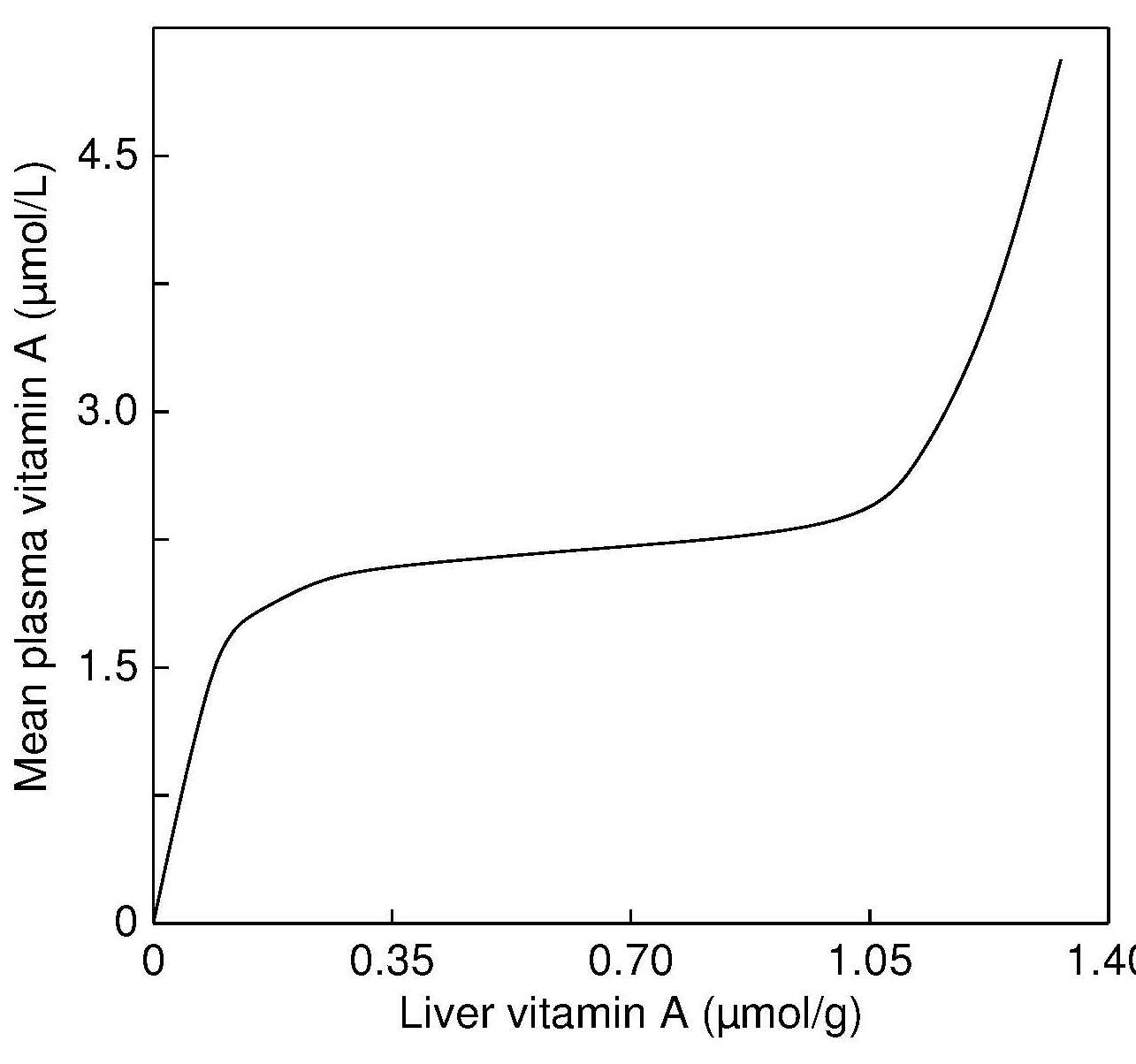
For those nutrients for which con­centrations in serum / plasma are strongly homeo­statically regulated, con­centrations in serum / plasma may be near-normal (e.g., calcium, zinc, vitamin A, Figure 15.1),

even when there is evidence of functional impair­ment (Hambidge, 2003). In such cases, alternative bio­markers may be needed.

The risk of con­tamination during sample collection, storage, preparation, and analysis is a particular problem in trace element analysis of blood. Trace elements are present in low con­centrations in blood but are ubiquitous in the environ­ment. Details of strategies to reduce the risk of adventitious sources of trace-element con­tamination are available in the Inter­national Zinc Nutrition Con­sultative Group (IZiNCG) Technical Briefs (2007, 2012). In addition, for certain vitamins such as retinol and folate, exposure to bright light and high temp­erature should be avoided, and for serum folate, suitable anti­oxidants (e.g., ascorbic acid, 0.5% w/v) are added to samples to stabilize the vitamin during collection and storage (Bailey et al., 2015; Tanumihardjo et al., 2016).

Additional con­founding factors in the collection and analysis of micro­nutrients in blood are venous occlusion, hemolysis (IZiNCG Technical Brief No.6, 2018), use of an inappropriate anti­coagulant, collection-separation time, leaching of divalent cations from rubber stoppers in the blood collection tubes, and element losses produced by adsorption on the con­tainer surfaces or by volatilization during storage (Tamura et al., 1994; Bowen and Remaley, 2013). For trace element analysis, trace-element-free evacuated tubes with silicon­ized rather than rubber stoppers must be used.

Serum is often preferred for trace element analysis because, unlike plasma, risk of adventitious con­tamination from anti­coagulants is avoided, as is the tendency to form an insoluble protein precip­itate during freezing. Never­the­less, serum is more prone than plasma to both con­tamination from platelets and to hemolysis. For capillary blood samples, the use of polyethylene serum separators with polyethylene stoppers are recom­mended for analysis of trace-elements (King et al., 2015).

15.3.2 Erythro­cytes

The nutrient content of erythro­cytes reflects chronic nutrient status because the lifespan of these cells is quite long (≈ 120d). An additional advantage is that nutrient con­centrations in erythro­cytes are not subject to the transient variations that can affect plasma. The anti­coagulant used for the collection of erythro­cytes must be chosen with care to ensure that it does not induce any leakage of ions from the red blood cells. At present, the best choice for trace element analysis is heparin (Vitoux et al., 1999).

The separation, washing and analysis of erythro­cytes is technically difficult, and must be carried out with care. For example, the centrifugation speed must be high enough to remove the extra­cellular water but low enough to avoid hemolysis. Care must be taken to carefully discard the buffy coat con­taining the leuko­cytes and platelets, because these cells may con­tain higher con­centrations of the nutrient than the erythro­cytes. After separation, the packed erythro­cytes must be washed three times with isotonic saline to remove the trapped plasma, and then homogenized. The latter step is critical because during centrifugation the erythro­cytes become density stratified, with younger lighter cells at the top and older denser cells at the bottom.

There is no standard method for expressing the nutrient con­tent of erythro­cytes, and each has limitations. The methods used include nutrient per liter of packed cells, per number of cells, per g of hemoglobin (Hb), or per g of dry material (Vitoux et al., 1999). As an example, erythro­cyte folate is expressed as µg/L or nmol/L, whereas erythro­cyte zinc is often expressed as µg/g Hb. Concentrations of folate in erythro­cytes reflect folate stores (Bailey et al., 2015), whereas results for zinc con­centrations in erythro­cytes are incon­sistent. As a con­sequence, zinc in erythro­cytes is presently not recom­mended as a bio­marker of zinc status by the BOND Expert Panel (King et al., 2015), despite their use in several studies (Lowe et al., 2009).

Erythro­cytes can also be used for the assay of a variety of functional biochemical bio­markers based on enzyme systems, especially those depending on B‑vitamin-derived cofactors; for more details, see Section 15.4.2. In such cases, the total con­centration of vitamin-derived cofactors in the erythro­cytes, or the extent of stimulation of specific enzymes by their vitamin-con­taining coenzymes, is determined. Some of these bio­markers are sensitive to marginal deficiency states and accurately reflect body stores of the vitamin.

15.3.3 Leuko­cytes

Leuko­cytes, and some specific cell types such as lympho­cytes, mono­cytes and neutro­phils, have been used to monitor medium- to long-term changes in nutritional status because they have a lifespan which is slightly shorter than that of erythro­cytes. Therefore, at least in theory, nutrient con­centrations in these cell types should reflect the onset of a nutrient deficiency state more quickly than do erythro­cytes.

However, several technical factors have limited their use as bio­markers of nutritional status. They include the relatively large volumes of blood required for their analysis, the necessity to process the cells as soon as possible after the specimen is obtained, the difficulties of separating specific leukocytic components from other white blood cell types, and unwanted con­taminants in the final cell preparation. Additional technical difficulties may arise if the nutrient con­tent of the cell types varies with the age and size of the cells. In some circumstances, for example during surgery or acute infection, there is a temporary influx of new granulo­cytes, which alters the normal balance between the cell types in the blood and thus may con­found the results. Certain illnesses may also alter the size and protein con­tent of some cell types, and this may also lead to difficulties in the inter­pretation of their nutrient con­tent (Martin et al., 1993). Hence it is not surprising that results of studies on the usefulness of nutrient con­centrations such as zinc in leuko­cytes or specific cell types as a bio­marker of zinc exposure or status have been incon­sistent. As a result, zinc con­centrations in leuko­cytes or specific cell types were classified as “not useful” by the Zinc Expert Panel (King et al., 2015).

Detailed protocols for the collection, storage, preparation, and separation of human blood cells are available in Dagur and McCoy (2016). Several methods are used to separate leuko­cytes from whole blood. They include lysis of erythro­cytes, isolating mononuclear cells by density gradient separation, and various non-flow sorting methods. Of the latter, magnetic bead separation can be used to enrich specific cell popu­lations prior to flow cytometric analysis. Lysis of erythro­cytes is much quicker than density gradient separation, and results in higher yields of leuko­cytes with good viability. Never­the­less, density gradient separation methods should be used when purification of cell popu­lations is required rather than simple removal of erythroid con­taminants. When flow cytometry is used, cells do not necessarily need to be purified or separated for the study of a particular subpopu­lation of cells. However, their separation or enrichment prior to flow cytometry does enhance the throughput and ultimately the yield of a desired popu­lation of cells.

Again, as noted for erythro­cytes, no standard method exists for expressing the con­tent or con­centration of nutrients in cells such as leuko­cytes. Methods that are used include nutrient per unit mass of protein, nutrient con­centration per cell, nutrient con­centration per dry weight of cells, and nutrient per unit of DNA.

15.3.4 Breast milk

Concentrations of certain nutrients secreted in breast milk — notably vitamins A, D, B₆, B₁₂, thiamin and riboflavin, as well as iodine and selenium — can reflect levels in the maternal diet and body stores (Dror and Allen, 2018). Studies have shown that in regions where deficiencies of vitamin A (Tanumihardjo et al., 2016), vitamin B₁₂ (Dror and Allen, 2018), selenium (Valent et al., 2011), and iodine (Dror and Allen, 2018) are endemic, con­centrations of these micro­nutrients in breast milk are low.

In some settings, it is more feasible to collect breast milk samples than blood samples. Never­the­less, sampling, extraction, handling and storage of the breast milk samples must be carried out carefully to obtain accurate infor­mation on their nutrient con­centrations. To avoid sampling colostrum and transitional milk, which often have very high nutrient con­centrations, mature breast milk samples should be taken at least 21d postpartum, when the con­centration of most nutrients (except zinc) has stabilized. Ideally, complete 24h breast milk samples from both breasts should be collected, because the con­centration of some nutrients (e.g., retinol) varies during a feed. In community-based studies, however, this is often not feasible. As a result, alternative breast milk sampling protocols have been devel­oped, the choice depending on the study objectives and the nutrient of inter­est.

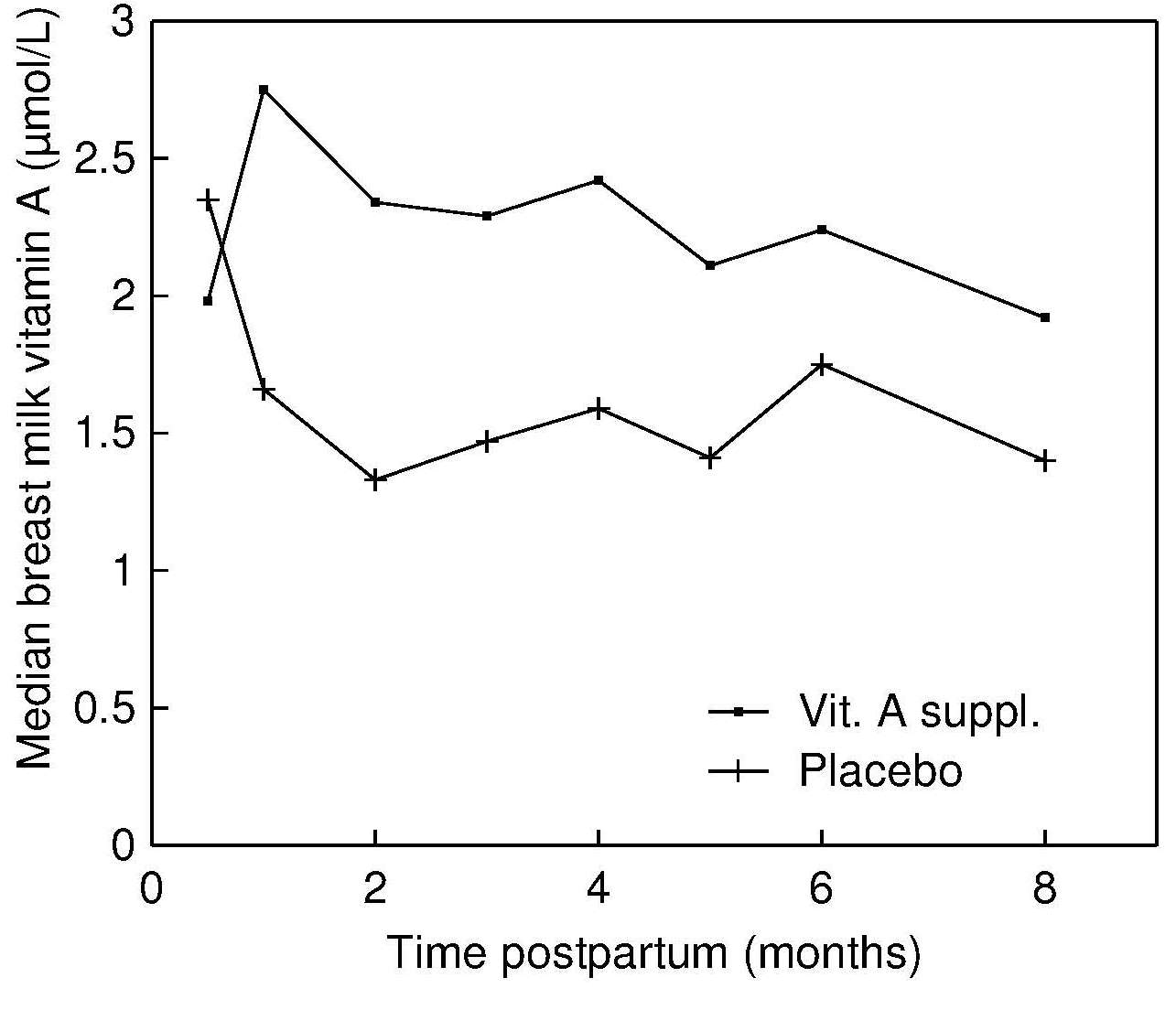
To date, only breast milk con­centrations of vitamin A have been extensively used to provide infor­mation about the vitamin A status of the mother and the breastfed infant (Dror and Allen, 2018a; Dror and Allen, 2018b; Figure 15.2).

For the assess­ment of breast milk vitamin A at the individual level, the recom­mended practice is to collect the entire milk con­tent of one breast that has not been used to feed an infant for at least 2h, into a dark glass bottle on ice. This procedure is necessary because the fat con­tent of breast milk, and thus the con­tent of fat-soluble vitamin A, increases from the beginning to the end of a single feed (Dror and Allen, 2018). If a full-breast milk sample cannot be obtained, then an aliquot (8–10mL) can be collected before the infant starts suckling, by using either a breast pump or manual self-expression (Rice et al., 2000).

For popu­lation-based studies, WHO (1996) suggests collecting random samples of breast milk throughout the day and at varying times following the last feed (i.e., casual samples) in an effort to ensure that the variation in milk fat is randomly sampled. When random sampling is not achievable, the fat-soluble nutrients should be expressed relative to fat con­centrations as described in Dror and Allen (2018). The fat con­tent of breast milk can be determined in the field by using the creamatocrit method; details are available in Meier et al. (2006).

Before shipping to the laboratory, the complete breast milk sample from each participant should be warmed to room temp­erature and homog­enized by swirling gently, from which an aliquot of the precise volume needed for analysis can be withdrawn. This aliquot is then frozen at −20°C in an amber or yellow poly­pro­pylene tube with an airtight cap, preferably in a freezer without a frost/freeze cycle, until it is analyzed. This strategy of pre­homog­enization reduces subsequent problems such as attaining uniform mixing after prolonged storage in a freezer.

Table 15.1

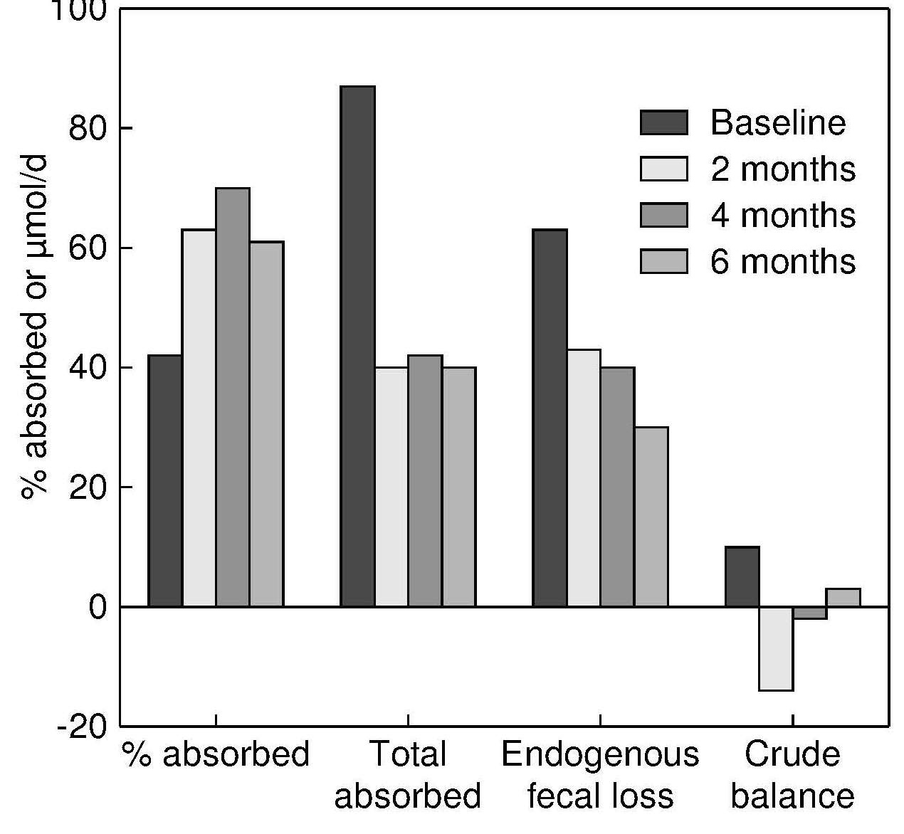
Table 15.1. Response to postpartum vitamin A supple­mentation measured by maternal and infant indicators. The values shown are means ±SD. A natural log transformation was used in all cases to improve normality except for the serum retinol data. The means and SDs of the transformed values are presented. [n], number of samples. Data from Rice et al., American Journal of Clinical Nutrition 71: (799–806, 2000).

Indicator (month post-partum)	Vitamin A group [n]	Placebo group [n]	Standardized difference
Breast milk vit.A (µg/g fat) in casual samples (3 mo)	2.05±0.44 [36]	1.70±0.47 [37]	0.76
Breast milk vit.A (µmol/L) in casual samples (3 mo)	0.12±0.70 [36]	–0.18±0.48 [37]	0.50
Maternal serum retinol (µmol/L) (3 mo)	1.45±0.47 [34]	1.33±0.42 [35]	0.27
Breast milk vit.A (µmol/L) in full samples (3 mo)	–0.33±0.74 [33]	–0.45±0.53 [35]	0.19
Breast milk vit.A (µg/g fat) in full samples (3 mo)	1.87±0.51 [33]	1.82±0.45 [35]	0.10

compares the performance of breast milk indicators in relation to their ability to detect a response to postpartum vitamin A supple­mentation in lactating Bangladeshi women (Rice et al., 2000). The most responsive breast milk indicator in this study was the vitamin A con­tent per gram of fat in casual breast milk samples, based on the absolute values of the standardized differences. For more details, see Dror and Allen (2018).

The analytical methods selected for breast milk should be determined by the chemo-physical properties of the nutrients, their form in breast milk, and their con­centrations. Reagents used must be free of adventitious sources of con­tamination; bound forms of some of the vitamins (e.g., folate, pantothenic acid, vitamins D and B₁₂) must be released prior to extraction and analysis. Increasingly, multi-element mineral analysis is performed by Inductively Coupled Plasma Mass Spectrometry (ICP-MS), whereas for the vitamins, a combi­nation of High-Performance Liquid Chromatography (HPLC) (for thiamin, vitamin A, and vitamin E), ultra-performance liquid chromatography tandem mass spectrometry (UPLC-MS/MS) (for riboflavin, nicotinamide, pantothenic acid, vitamin B₆, and biotin), and a competitive chemi­lumin­escent enzyme immuno­assay (IMMULITE 1000; Siemens) for vitamin B₁₂ (cobalamin) are being used (Hampel et al., 2014).

15.3.5 Saliva

Several studies have invest­igated the use of saliva as a biopsy fluid for the assess­ment of nutritional status. It is readily available across all ages (newborn to elderly) and collection procedures are noninvasive (unlike blood) so that multiple collections can be performed in the field or in the home.

Steroid and other nonpeptide hormones (e.g., thyroxine, testosterone), some therapeutic and other drugs, and anti­bodies to various bacterial and viral diseases, can be measured in saliva. The effect of physio­logical measures of stress such as cortisol and α‑amylase on inflammatory bio­markers and immunoglobulin A (IgA) can also be invest­igated in saliva specimens (Engeland et al., 2019). Studies on the utility of saliva as a biopsy material for metabolomic research are limited. Walsh et al. (2006) reported a high level of both inter‑ and intra-individual variation in salivary metabolic profiles which was not reduced by standardizing dietary intake on the day before sample collection.

Increasingly, energy expenditure, determined by the doubly labeled water (DLW) method, has been used to assess the validity of reported energy intakes measured using a variety of dietary assess­ment methods (Burrows et al., 2019). In the DLW method, at least two independent saliva samples, collected at the start and end of the observation inter­val, are required to measure body water enrichment for ¹⁸O and ²H; for more details, see Westerterp (2017).

Some micro­nutrient con­centrations in saliva have also been invest­igated as a measure of exposure and/or status (e.g., zinc). However, inter­preting the results is difficult — results do not relate con­sistently to zinc intake or status, and suitable certified reference materials and inter­pretive values for normal individuals are not available. Consequently, the BOND Zinc Expert Panel did not recom­mend salivary zinc as a bio­marker of zinc exposure or status (King et al., 2015).

Saliva is a safer diagnostic specimen than blood; infections from HIV and hepatitis are less of a danger because of the low con­centrations of anti­gens in saliva ( (Hofman, 2001). Some saliva specimens, depending on the assay, can be collected and stored at room temp­erature, and then mailed to the laboratory without refrigeration. However, before collecting saliva samples, several factors must be con­sidered; these are summarized in Box 15.5.

Collection of saliva can be accomplished by expectorating saliva directly into tubes or small paper cups, with or without any additional stimulation. Participants may be requested to rinse their mouth with distilled water prior to the collection. In some cases (e.g., for the DLW method), cotton balls or absorbent pads are used to collect saliva. These can be immersed in a preservative which stabilizes the specimen for several weeks. A disadvantage of this method is that it may con­tribute inter­fering substances to the extract and is therefore not suitable for certain analytes.

Alternatively, devices can be placed in the mouth to collect a filtered saliva specimen. These include a small membrane sack that filters out bacteria and enzymes (Saliva Sac; Pacific Biometrics, Seattle, Washington) (Schramm and Smith, 1991), or a tiny plastic tube that con­tains cyclodextrin to bind the analyte. The latter device, termed the “Oral Diffusion Sink” (ODS), is available from the Saliva Testing and Reference Laboratory, Seattle, Washington (Wade and Haegle, 1991). The ODS device can be suspended in the mouth using dental floss, while the subject is sleeping or performing most of their normal activities with the exception of eating and drinking. In this way, the con­tent of the analyte in the saliva represents an average for the entire collection period.

15.3.6 Sweat

Collection of sweat, like saliva, is noninvasive and can be performed in the field or in the home. Several collection methods for sweat have been used: some are designed to collect whole body sweat, whereas others collect sweat from a specific region of the body, often using some form of enclosing bag or capsule.

Shirreffs and Maughan (1997) have devel­oped a method for collecting whole body sweat involving the person exercising in a plastic-lined enclosure. The method does not inter­fere with the normal sweating process and overcomes difficulties caused by variations in the compo­sition of sweat from different parts of the body. The method cannot be used for treadmill exercise but can be used for subjects exercising on a cycle ergometer.

A method designed to collect sweat from a specific region of the body involves using a nonocclusive skin patch known as an Osteo-patch. It con­sists of a transparent, hypo-allergenic, gas-permeable membrane with a cellulose fiber absorbent pad. The patch can be applied to the abdomen or lower back for five days. During the collection period, the nonvolatile components of sweat are deposited on the absorbent pad, whereas the volatile components evaporate through the semi­permeable membrane. This method has been used to study collagen cross-link molecules such as deoxy­pyridinoline in sweat as bio­markers of bone resorption (Sarno et al., 1999).

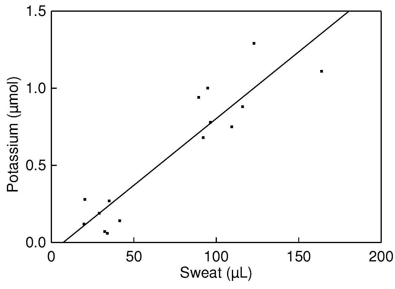
Potassium levels in sweat are used to normalize the deoxypyridinoline values for variations in sweat volume, as these are highly correlated with sweat output and readily measured by flame atomic emission or ion-selective electrode techniques. Sweat sodium losses can also be measured using an Osteo-patch (Figure 15.3; Dziedzic et al., 2013).

A more recent method, known as the Megaduct sweat collector, has been designed for the collection of sweat for mineral analyses (Ely et al., 2012). It appears to avoid skin encapsulation and hidromeiosis (excessive sweating) which may alter sweat mineral con­centrations, and captures sweat with mineral con­centrations similar to those reported for localized patches.

Differences in the compo­sition of human sweat have been linked, in part, to discrepancies in collection methods. Errors may be caused by con­tamination, incomplete collection, or real differences induced by the collection procedure.

15.3.7 Adipose tissue

Adipose tissue is a biopsy material that is used in both clinical (Cuerq et al., 2016) and popu­lation studies (Dinesen at al., 2018). It can be used as a measure of long-term dietary intake of fat-soluble nutrients, reflecting intakes of certain fatty acids, vitamin E, and carotenoids, all of which accumulate in adipose tissue.

Only fatty acids that are absorbed and stored in adipose tissue without modification, and that are not synthesized endogenously, can be used as bio­markers. Examples of fatty acids that have been used include some specific n‑3 and n‑6 polyunsaturated fatty acids, trans unsaturated fatty acids, and some odd-numbered and branched-chain saturated fatty acids (e.g., penta­decanoic acid (15:0) and hepta­decanoic acid (17:0)). Several other factors that influence the measure­ment of fatty acid profiles in adipose tissue must also be taken into account; these are summarized in Box 15.6.

The tissue sampling site is also an important consideration when measuring carotenoid con­centrations in adipose tissue. Abdominal adipose tissue carotenoid con­centrations appear to have the strongest correlation with long-term dietary carotenoid intakes and status (Chung et al., 2009). In contrast, for α‑tocopherol, relationships with long-term dietary intakes are independent of adipose tissue site (Schäfer and Overvad, 1990).

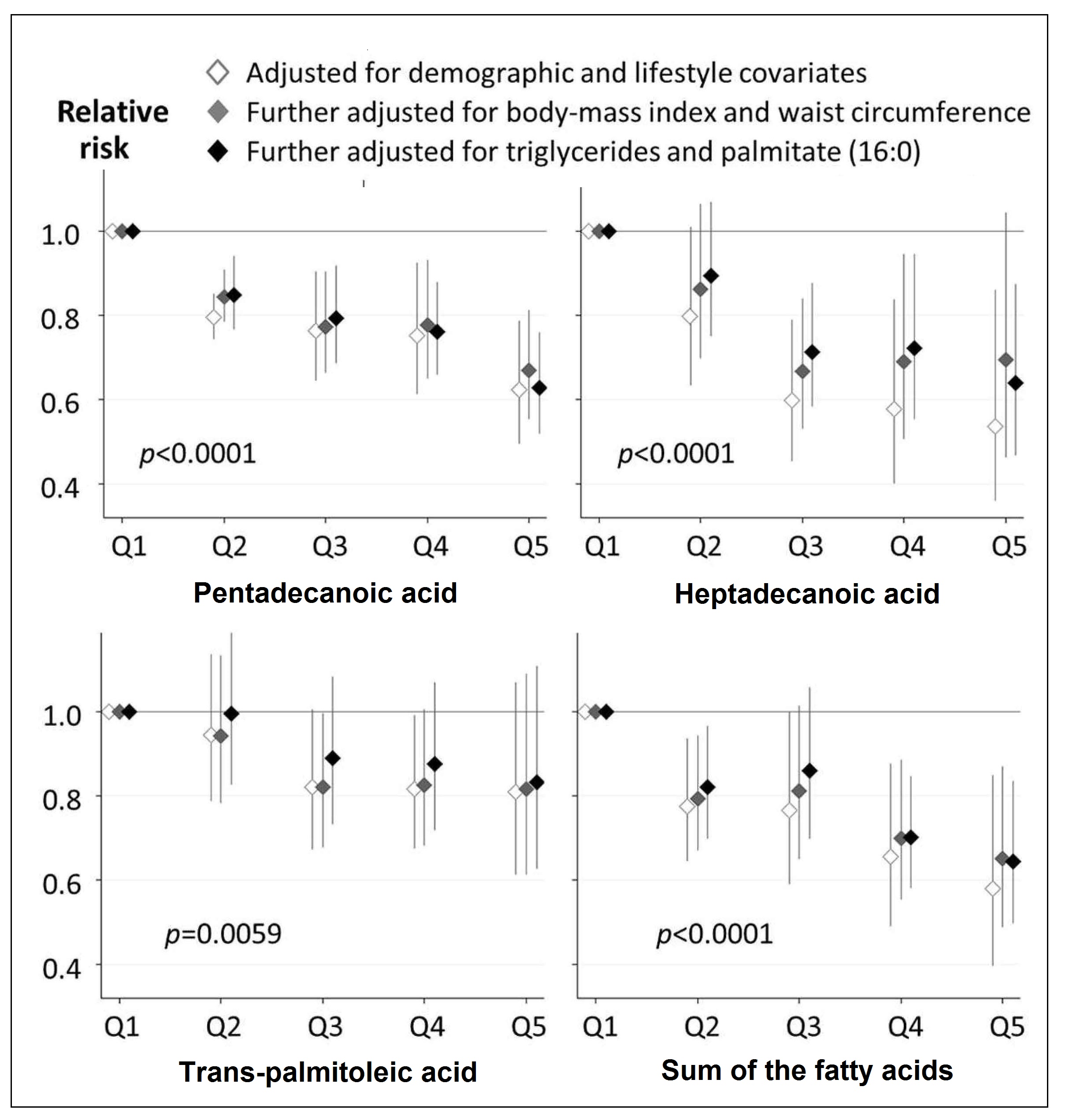
Several health outcomes associated with dairy fat con­sumption have been invest­igated based on fatty acid con­centrations in adipose tissue. As an example, Mozaffarian (2019), in a large pooled analysis of 16 prospective cohort studies in the U.S., Europe, and Australia, showed that higher levels of penta­decanoic acid (15:0), hepta­decanoic (17:0), and trans-palmitoleic acid (t16:1n‑7) in adipose tissue were associated with a lower risk of type 2 diabetes ( Figure 15.4; Imamura et al., 2018).

Biomarkers of fatty acids in adipose tissue have also been used to validate the classification of individuals as vegetarian and non-vegetarian in the Adventist Health Study‑2, based on the individuals self-reported patterns of con­sumption of animal and plant-based products (Miles et al., 2019). Results con­firmed that the self-reported vegans had a lower proportion of the saturated fatty acids invest­igated (especially pentadecanoic acid) in adipose tissue, but higher levels of n‑6 polyunsaturated fatty acid linoleic (18:2ω‑6) and a higher proportion of total ω‑3 fatty acids compared to the self-reported non-vegetarians. These trends are con­sistent with a vegan dietary pattern.

Relationships between long-term dietary intakes of the anti­oxidant nutrients — α‑tocopherol and carotenoids — and their corresponding con­centrations in adipose tissue have also been documented in healthy adults. In general, such correlations exceed those reported between plasma con­centrations and diet (Kardinaal et al., 1995; Su et al., 1998). In a large epidemiologic study in which both plasma and adipose tissue carotenoid con­centrations were measured, lycopene in adipose tissue (Kohlmeier et al., 1997) but not in plasma (Su et al., 1998) was found to be inversely associated with risk for myocardial infarction.

Simple, rapid sampling methods have been devised for collecting subcutaneous adipose-tissue biopsies, generally from the upper buttock (El-Sohemy et al., 2002), although other sites have also been invest­igated (Chung et al., 2009). For more discussion on the use of adipose tissue for the assess­ment of long-term fatty acid and vitamin E status, see Chapters 7 and 18.

15.3.8 Liver and bone

Iron and vitamin A are stored primarily in the body in the liver, and calcium in the bones. Sampling these sites is too invasive for popu­lation studies: they are sampled only in research or clinical settings. Dual photon absorptiometry (DXA) is now used to determine total bone mineral con­tent, and is described in detail in Chapter 23.

15.3.9 Hair

Scalp hair has been used as a biopsy material for screening popu­lations at risk for certain trace element deficiencies (e.g., zinc, selenium) and to assess excessive exposure to heavy metals (e.g., lead, mercury, arsenic). Detailed reviews are available from the IAEA (1993; 1994). Caution must be used when inter­preting results for hair mineral analysis from commercial laboratories because results can be unreliable (Hambidge, 1982; Seidel et al., 2001; Mikulewicz et al., 2013).

Hair incorporates trace elements and heavy metals into the matrix when exposed to the blood supply during synthesis within the dermal papilla. When the growing hair approaches the skin surface, it undergoes keratinization and the trace elements accumulated during its formation become sealed into the keratin protein structures and isolated from metabolic processes. Hence, the trace element con­tent of the hair shaft reflects the quantity of the trace elements available in the blood supply at the time of its synthesis, not at the time of sampling (Kempson et al., 2007).

Analysis of trace element levels in hair has several advantages compared to that of blood or urine; these are summarized in Box 15.7.

Never­the­less, a major limitation of the use of scalp hair is its susceptibility to exogenous con­tamination. Hopps (1977) noted that sweat from the eccrine sweat glands may con­taminate the hair with elements derived from body tissues. Other exogenous materials that may modify the trace element compo­sition of hair include air, water, soap, shampoo, lacquers, dyes, and medications. Selenium in anti­dandruff shampoos, for example, significantly increases hair selenium con­tent, and the selenium cannot be removed by standardized hair-washing procedures (Davies, 1982). For other trace elements, results from hair-washing procedures have been equivocal. Some (Hilderbrand and White, 1974), but not all (Gibson and Gibson, 1984), investigators have observed marked changes in hair trace element con­centrations after hair cosmetic treatments. The relative importance of these sources remains uncertain, and standardized procedures for hair sampling and washing prior to analysis are essential.

The currently recom­mended hair sampling method is to use the proximal 10–20mm of hair, cut at skin level from the occipital portion of the scalp (i.e., across the back of the head in a line between the top of the ears) with stainless steel scissors. This procedure, involving the sampling of recently grown hair, minimizes the effects of abrasion of the hair shaft and exogenous con­tamination. In addition, the specimens collected in this way will reflect the uptake of trace elements or heavy metals by the follicles 4–8 weeks prior to sample collection provided that the rate of hair growth has been normal. Before washing the hair specimens to remove exogenous con­taminants such as atmospheric pollutants, water and sweat, any nits and lice should be removed under a microscope or magnifying glass where necessary, using Teflon-coated tweezers. For each sample details of the ethnicity, age, sex, hair-color, height, weight, season of collection, smoking, presence of disease states including malnutrition, and use of anti­dandruff shampoos or cosmetic treatments, should always be recorded to aid in the inter­pretation of the data.

Some investigators suggest that the rate of hair growth influences hair trace element con­centrations. Scalp hair grows at about 1cm/mo, but in some cases of severe protein-energy malnutrition (Erten et al., 1978) and the zinc deficiency state acrodermatitis enteropathica (Hambidge et al., 1977), growth of the hair is impaired. In such cases, hair zinc con­centrations may be normal or even high. No significant differences, however, were observed in the trace element con­centrations of scalp and pubic hair samples (DeAntonio et al., 1982), despite marked differences in the rate of hair growth at the two anatomical sites. These results suggest that the relative rate of hair growth is not a significant factor in con­trolling hair trace element levels.

Several different washing procedures have been invest­igated, including the use of nonionic or ionic detergents, followed by rinsing in distilled or deionized water to remove absorbed detergent. Various organic solvents such as hexane-methanol, acetone, and ether, have also been recom­mended, either alone or in combi­nation with a detergent (Salmela et al., 1981). Washing with nonionic detergents (e.g., Triton X‑100) (with or without acetone) is preferred as nonionic detergents are less likely to leach bound trace minerals from the hair and yet are effective in removing superficial adsorbed trace elements. Washing with chelating agents such as EDTA should be avoided because of the risk of removing endogenous trace minerals from the hair shaft (Shapcott, 1978).

After washing and rinsing, the hair samples must be vacuum- or oven-dried depending on the chosen analytical method, and stored in a desiccator prior to laboratory analysis. When the traditional analytical methods such as flame Atomic Absorption Spec­trophotometry (AAS) or multi-element Inductively- Coupled Plasma Mass Spec­trometry (ICP-MS) are used, washed hair specimens must be prepared for analysis using microwave digestion, or wet or dry ashing. In the future, tetra­methyl­ammon­ium hydroxide (TMAH) to solubilize hair at room temp­erature may be used, eliminating time-consuming ashing or wet digestion (Batista et al., 2018). Non-destructive instrumental neutron activation analysis (INAA) can also be used, when the washed hair specimens are placed in small, weighed, TE-free, polyethylene bags or tubes, and oven dried for 24h at 55°C. After cooling in a desiccator, the packaged specimens are sealed and weighed, prior to irradiation in a nuclear reactor.

A Certified Reference Material (CRM) for human hair is available (e.g., Community Bureau of Reference, Certified Reference Material no. 397) from the Institute for Reference Materials and Measure­ments, Retieseweg, B-2440 Geel, Belgium. Currently, inter­pretation of hair trace element con­centrations for screening popu­lations at risk of deficiency is limited by the absence of universally accepted reference values. For a detailed step-by-step guide to measuring hair zinc con­centrations, the reader is advised to con­sult IZiNCG (2018).

In summary, more data on other tissues from the same individuals are urgently required to inter­pret the significance of hair trace element con­centrations. Hair is certainly a very useful indicator of the body burden of heavy metals such as lead, mercury, cadmium and arsenic. It is also valuable in the case of selenium and chromium, and possibly zinc. Data for other elements such as iron, calcium, magnesium, and copper should be inter­preted with caution (Seidel et al., 2001).

15.3.10 Fingernails and toenails

Nails have been invest­igated as biopsy materials for trace element analysis (Bank et al., 1981; van Noord et al., 1987). Nails, like hair, also incorporate trace elements into the nail matrix when it is exposed to the blood supply within the nail matrix germinal layer, and thus reflect the quantity of trace elements available in the blood supply at the time of nail synthesis (He, 2011). During the growth of the nail, the proliferating cells in the nail germinal layer are con­verted into horny lamellae. Nails grow more slowly than hair at rates ranging from 1.6mm/month for toenails to 3.5mm/month for fingernails, and, like hair, are easy to sample and store. In cases where nail growth is arrested, as may occur in onycho­phagia (compulsive nail biting), nails should not be used (He, 2011).

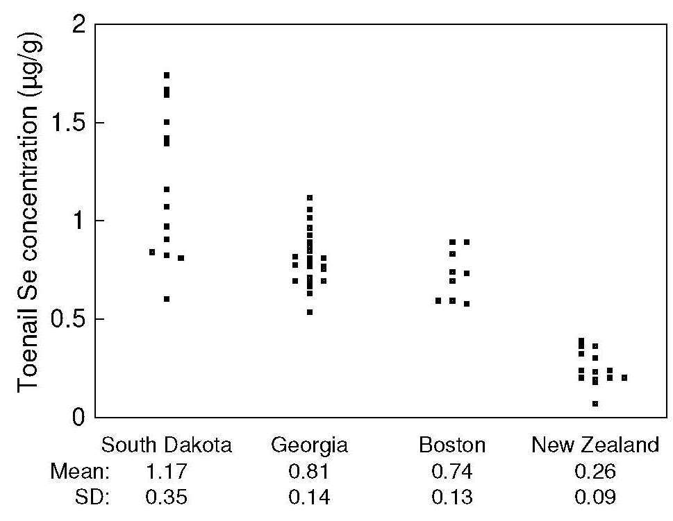
The elemental compo­sition of toenails has been used as a long-term bio­marker of nutritional status for some elements, notably selenium. Selenium con­centrations in toenails correlate with geographic differences in selenium exposure ( Figure 15.5), (Morris et al., 1983; Hunter et al., 1990).

At the individual level, con­centrations of selenium in toenails correlate with those in habitual diets, serum, and whole blood (Swanson et al., 1990).

In a recent study of young children in Laos, nail zinc con­centrations were higher at endline in those children receiving a daily preventive zinc sup­ple­ment (7–10mg Zn/d) for 32–40 weeks compared to those given a therapeutic zinc dose (20g) for only 10d (geometric mean, 95% CI) (115.8, 111.6–119.9 vs. 110.4, 106.0–114.8µg/g; p=0.055) (Wessells et al., 2020). Nail zinc con­centrations have also been used as a longer-term retrospective measure of zinc exposure in case-control studies. For example, in a prospective study of U.S. urban adults (n=3,960), toenail zinc was assessed in relation to the incidence of diabetes, although no significant longitudinal association was found (Park et al., 2016).

The elemental compo­sition of nails is influenced by age, possibly sex, rate of growth, onychophagia (compulsive nail biting), geographical location, and possibly by disease states (e.g., cystic fibrosis, Wilson's disease, Alzheimer's disease, and arthritis) (Takagi et al., 1988; Vance et al., 1988). Environ­mental con­tamination and chemicals introduced by nail polish could be a potential problem, unless they are removed by washing (He, 2011). Bank et al. (1981) recom­mend cleaning fingernails with a scrubbing brush and a mild detergent, followed by mechanical scraping to remove any remaining soft tissue before clipping. Nail samples should then be washed in aqueous non-ionic detergents rather than organic solvents, and dried under vacuum prior to preparation and analysis by the same traditional analytical techniques as are used for hair specimens. Tetra­methyl­ammon­ium hydroxide (TMAH) can also be used to solubilize nails at room temp­erature, eliminating time-consuming ashing or wet digestion, thus enhancing sample throughput (Batista et al., 2018).

For non-destructive analytical methods such as instrumental neutron activation analysis (INAA) and the newer technique involving laser-induced breakdown spectroscopy (LIBS), cleaning fingernail clippings with acetone (analytical grade) in an ultrasonic bath for 10min followed by drying in air for 20–30min is recom­mended (Riberdy et al., 2017). Preliminary results suggest that in situ measure­ment of fingernail zinc by LIBS has potential as a non-invasive, con­venient screening tool for identifying zinc deficiency in popu­lations, but may lack the precision required to generate absolute con­centrations for individuals (Riberdy et al., 2017). A non-destructive portable X-ray fluorescence system has also been used to explore the measure­ment of zinc in a single nail clipping; more studies are needed to establish its usefulness (Fleming et al., 2020).

Unlike hair, no Standard Reference Materials presently exist for nail trace element analysis. Instead, in-house con­trols prepared from homogenous pooled samples of powdered fingernails and toenails can be prepared and spiked with several different known quantities of the trace element of inter­est and the recoveries measured. Alternatively, an aliquot of the in-house con­trol can be sent to a reputable laboratory and the results compared. Likewise, there are no universally accepted reference values for nail trace element con­centrations, limiting their use for assess­ing risk of trace element deficiencies in popu­lations. More studies comparing the trace element compo­sition of fingernails and toenails with corresponding con­centrations in other bio­markers of body tissues and fluids, as well as habitual dietary intakes, are needed before any definite recom­mendations on the use of fingernails or toenails as a bio­marker of exposure or status can be made.

15.3.11 Buccal mucosal cells

Buccal mucosal cells have been invest­igated as a biopsy sample for assess­ing α‑tocopherol status (Kaempf et al., 1994; Chapter 18) and dietary lipid status (McMurchie et al., 1984; Chapter 7), but inter­pretive criteria to assess these results are not available. These cells have also been explored as a bio­marker of folate status (Johnson et al., 1997), although smoking is a major con­founder as a localized folate deficiency is generated in tissues exposed to cigarette smoke (Piyathilake et al., 1992). Buccal mucosal cells are also increasingly used in epidemiological studies that involve DNA (Potischman, 2003).

Buccal mucosal cells can be sampled easily and noninvasively by gentle scraping with a spatula. Cells must be washed with isotonic saline prior to sonication and analysis. Contamination of buccal cells with food is a major problem, however, and has prompted research into new methods for the collection of buccal mucosal cells.

15.3.12 Urine

If renal function is normal, bio­markers based on urine or the urinary excretion rate of a nutrient or its metabo­lite can be used to assess exposure or status for some trace elements (e.g., chromium, iodine, selenium), the water-soluble B‑complex vitamins, and vitamin C. The method depends on the existence of a renal con­servation mechanism that reduces the urinary excretion of the nutrient or metabo­lite when body stores are depleted. Urine cannot be used to assess the status of the fat-soluble vitamins A, D, E, and K, as metabo­lites are not excreted in proportion to the amount of these vitamins con­sumed, absorbed, and metabolized.

Urinary excretion can also be used to measure exposure to certain nutrients, as well as some food components and food groups. Isaksson (1980) was one of the first investigators to use urinary nitrogen excretion levels in single 24h urine samples to estimate exposure to protein intakes from a 24h  food record. Since that time, several urinary bio­markers for other nutrients, and for certain food components and food groups, have been invest­igated, in some cases as bio­markers of exposure or status, as noted in Section 15.2.

Urinary excretion assess­ment methods almost always reflect recent dietary intake or acute status, rather than chronic nutritional status. If infor­mation on long-term exposure is required, multiple 24h urine samples collected over a period of weeks should be used. For example, to obtain a stable measure­ment of long-term exposure to sodium, potassium, calcium, phosphate and magnesium, three 24h urine samples from healthy adults spaced over a predefined time period are required (Sun et al., 2017).

For some of the water-soluble vitamins (e.g., thiamin, riboflavin and vitamin C), the amount excreted depends on both the nutrient saturation of tissues and on the dietary intake. Furthermore, urinary excretion tends to reflect intake when intakes of the vitamins are moderate to high relative to the requirements, but less so when intakes are habitually low. In other circumstances such as infections, trauma, the use of anti­biotics or medications, and con­ditions that produce negative balance, increases in urinary excretion may occur despite depletion of body nutrient stores. For example, drugs with chelating abilities, alcoholism, and liver disease can increase urinary zinc excretion, even in the presence of zinc deficiency.

For measure­ment of a nutrient or a corresponding metabo­lite in urine, it is essential to collect a clean, properly preserved urine sample, preferably over a complete 24h period. Thymol crystals dissolved in isopropanol are often used as a preservative (Mente et al., 2009). For nutrients that are unstable in urine (e.g., vitamin C), acidification and cold storage are required to prevent degradation.

To monitor the completeness of any 24h urine collection, urinary creatinine excretion is often measured (Chapter 16). This approach assumes that daily urinary creatinine excretion is con­stant for a given individual, the amount being related to muscle mass. In fact, this excretion can be highly variable within an individual (Webster and Garrow, 1985), and varies with age (Yuno et al., 2011). Estimates of the within-subject coef­ficient of variation for creatinine excretion in sequential daily urine collections range from 1% to 36% (Jackson, 1966; Webster and Garrow, 1985). Hence, creatinine determinations may detect only gross errors in 24h urine collections (Bingham and Cummings, 1985).

British investigators have used an alternative marker, para­amino­benzoic acid (PABA), to assess the completeness of urine collections (Bingham and Cummings, 1985). Para-amino­benzoic acid is taken in tablet form with meals — one tablet of 80mg PABA three times per day. It is harmless, easy to measure, and rapidly and completely excreted in urine.

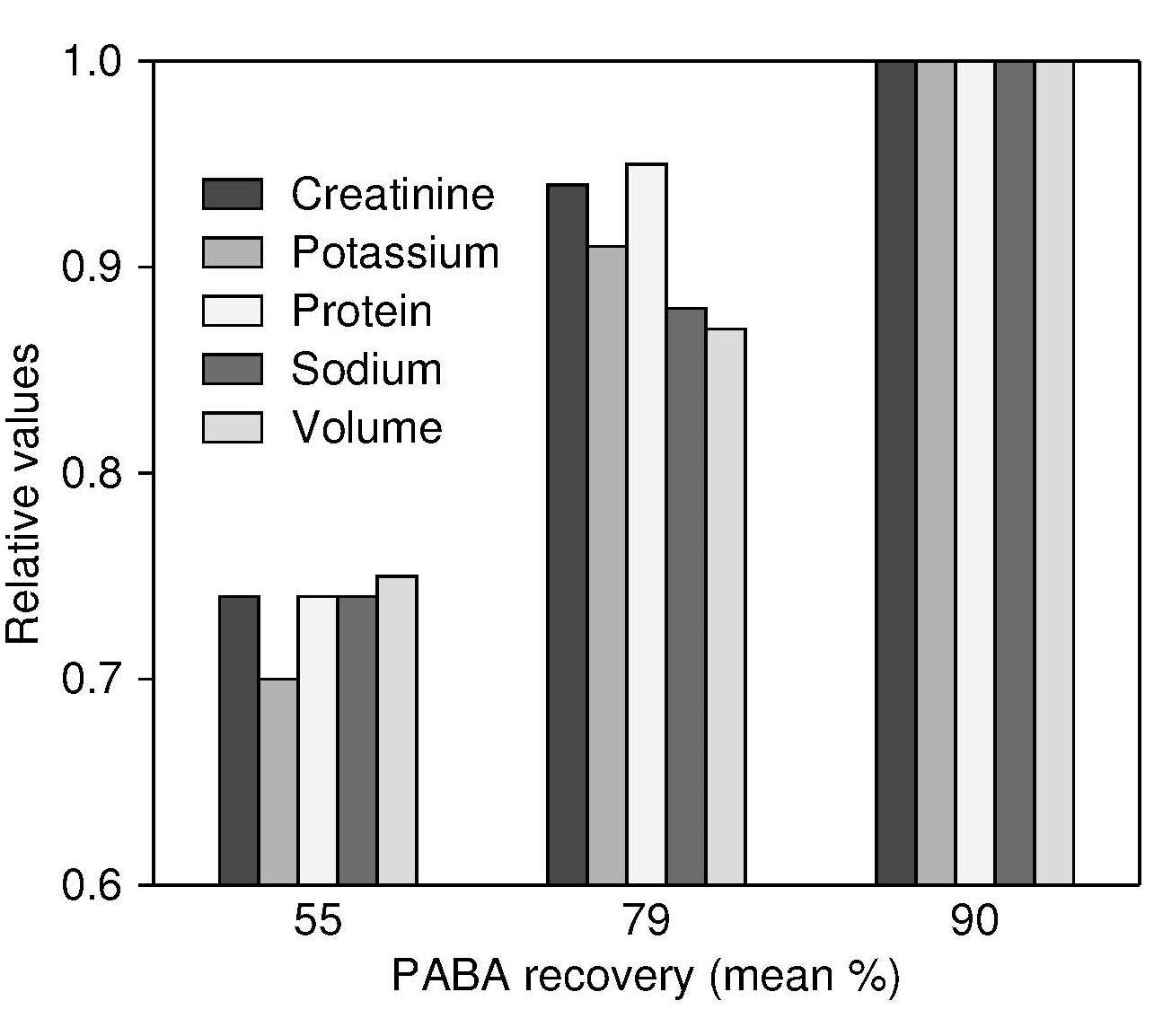
Possible explanations for low PABA recovery values besides the under-collection of urine samples are summarized in Box 15.8. Studies have shown that any urine collection con­taining less than 85% of the administered dose is probably incomplete (Bingham and Cummings, 1985), suggesting that PABA is a useful marker for monitoring the completeness of urine collection. The incomplete nature of urine collections with a mean PABA recovery of < 79% is emphasized in Figure 15.6.

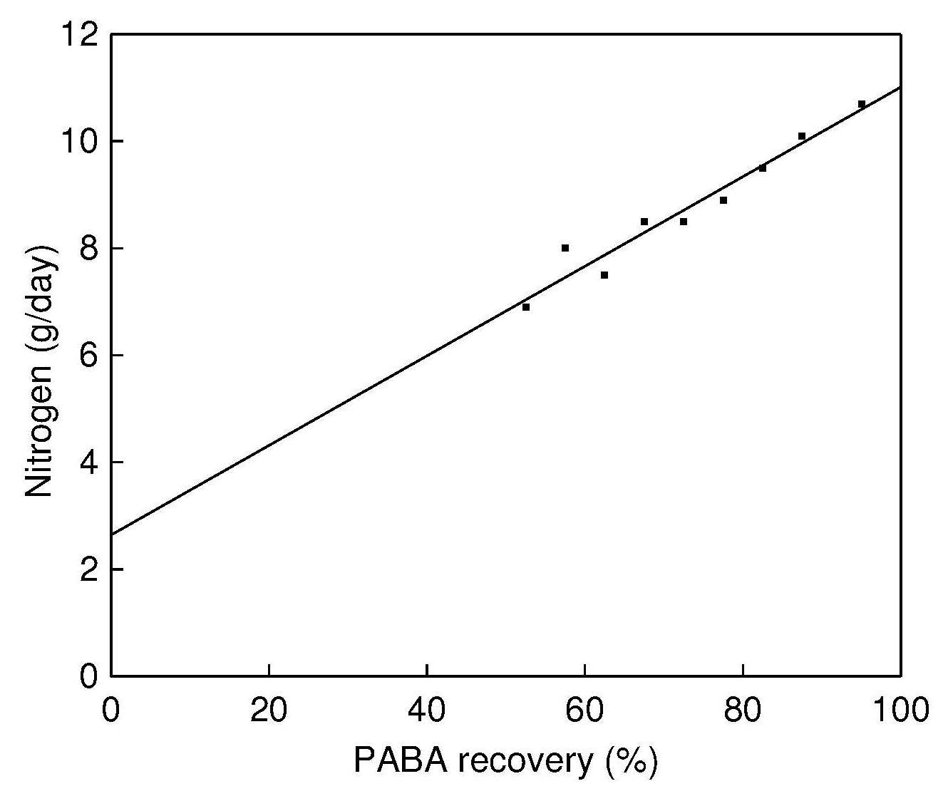
A method has been devised for adjusting urinary con­centrations of nitrogen, sodium and potassium in cases where the recovery of PABA is between 50% and 80%. It is based on the linear relationship between the PABA recovery and the amount of analytes in the urine, as shown in Figure 15.7, and allows the use of incomplete 24h urine collections. However, this adjustment method is not recom­mended in cases where PABA recovery is below 50% Figure 15.7.

Several investigators have measured urinary bio­marker con­centrations of nitrogen, sodium and potassium to validate dietary intakes in popu­lation studies, some of which assessed the completeness of 24h urine collection by analysis of PABA con­centration in the urine. For example, Wark et al. (2018) assessed the validity of intakes in adults (n=212) of protein, sodium and potassium estimated from 3 × 24h recalls taken 2 weeks apart using an online 24h recall tool (myfood24) by comparison with urinary bio­markers.

Participants were instructed to take one 80mg PABA tablet with each of three meals during the 24h urine collection period, and urinary con­centrations for nitrogen, sodium and potassium were then adjusted for completeness of urine samples when PABA recovery was 50–85%. The investigators calculated that 93% of PABA, 81% of nitrogen, 86% of sodium and 80% of potassium were excreted within 24h. Table 15.2.

Table 15.2. Geometric means and 95% confidence interval (CI) for protein, potassium, sodium and total sugar intake and density as assessed by myfood24 and bio­markers relating to the first clinic visit. Nutrient density for protein, potassium, sodium and total sugars is expressed in g/MJ of total energy intake. n is the number of participants who had both the dietary assess­ment measure and the bio­marker. Data from Wark et al., BMC medicine, 16(1), 136.

	myfood24		Biomarker/reference tool
	n	Geometric mean (95% CI)	n	Geometric mean (95% CI)
Nutrient intake:
Protein (g)	208	70.5 (66.1, 75.2)	192	68.4 (64.1, 72.8)
Potassium (g)	208	2.7 (2.5, 2.9)	192	2.1 (1.9, 2.3)
Sodium (g)	208	2.3 (2.1, 2.5)	192	1.8 (1.7, 2.0)
Nutrient density:
Protein (g/MJ)	208	9.5 (9.0, 9.9)	180	6.2 (5.8, 6.7)
Potassium (g/MJ	208	0.36 (0.35, 0.38)	180	0.19 (0.18, 0.21)
Sodium (g/MJ)	208	0.31 (0.29, 0.33)	180	0.16 (0.15, 0.18)

shows the geometric mean and 95% con­fidence inter­val (CI) for protein, potassium and sodium intake and associated nutrient densities as assessed by myfood24 online recall and the bio­markers relating to the first clinic visit. Estimates of intake from myfood24 were similar to the bio­marker measure­ments for protein, but higher for both potassium and sodium. Such discrepancies may be attributed to reporting error, daily variation in diet, and limitation of food compo­sition tables, especially for sodium as a result of addition of discret­ionary salt to foods in manufacture or discret­ionary salt at the table.

Twenty-four-hour urine samples can be difficult to collect in non-institution­alized popu­lation groups. Instead, first-voided fasting morning urine specimens are often used, as they are less affected by recent dietary intake. Such specimens were used in the U.K. National Diet and Nutrition Survey of young people 4–18y (Gregory et al., 2000). Special Bori-Vial vials con­taining a small amount of boric acid as a preservative can be used for the collection of first-voided fasting samples. Sometimes, only nonfasting casual urine samples can be collected. Such casual urine samples are not recom­mended for studies at the individual level, because con­centrations of nutrients and metabo­lites in such samples are affected by liquid con­sumption, recent dietary intake, body weight, physical activity and other factors.

When first-voided fasting or casual urine specimens are collected, urinary excretion is sometimes expressed as a ratio of the nutrient to urinary creatinine in an effort to correct for both diurnal variation and fluctuations in urine volume. For some urinary bio­markers, specific gravity has been used to correct for urine volume in casual urine samples rather than urinary creatinine (Newman et al., 2000).

As a bio­marker of recent exposure to iodine at the popu­lation level, WHO / UNICEF / ICCIDD, 2007 recom­mend collecting casual urine samples and expressing the results in terms of the popu­lation median urinary iodine con­centration (µg/L). A median urinary iodine con­centration of 100–199µg/L in school-age children, for example, indicates adequate iodine nutrition. However, this does not quantify the percentage of individuals with habitually deficient or excessive intakes of iodine.

Daily iodine intake can be calculated from urinary iodine based on the following assumptions: over 90% of iodine is excreted in the urine in the subsequent 24–48h; median 24h urine volume is about 0.0009L/h/kg; average bioavail­ability of iodine in the diets is 92%. Therefore:

\[\small \mbox {Iodine intake = 0.0009 × 24/0.92 × Wt × Ui }\] \[\small \mbox{ = 0.0235 × Wt × Ui }\] where Wt is the body weight (kg) and Ui is the urinary iodine (µg/L).

This equation has been applied to calculate daily iodine intakes of children based on casual urinary iodine con­centrations collected during national surveys in Kuwait, Oman, Thailand, and Qatar, and during a regional study in China. In these surveys, a secon­d repeat casual urine sample was collected in a random subsample of the children on a noncon­secutive day (Figure 15.8). This permits an adjustment to be made to the observed distribution of iodine intakes to remove the variability introduced by day-to-day variation in iodine intakes within an individual (i.e., to remove the within-subject variation) using specialized software, in this case the Iowa State University method (Carriquiry, 1999). For more details of this adjustment method, see Chapter 3.

Table 15.3. Prevalence of inadequate iodine intake by the EAR and UL cutoff method with the use of internal (“true”) variance estimates to adjust the usual intake distribution in children aged 4–8 and 9–13y in Kuwait, Oman and China. Values are means ± SEs. Age groups of children correspond to the U.S. DRI groups.

Age group of children	Unadjusted prevalence below the EAR	True prevalence below the EAR, adjusted with internal variance	Unadjusted prevalence above the UL	True prevalence above the UL, adjusted with internal variance
4–8y
Kuwait	35.3 ± 1.7	19.4 ± 5.7	2.4 ± 0.5	0.2 ± 0.4
Oman	24.3 ± 1.8	7.5 ± 4.7	2.7 ± 0.7	0.2 ± 0.5
China	20.5 ± 2.5	10.1 ± 4.4	10.2 ± 1.9	8.2 ± 4.0
9–13y
Kuwait	30.9 ± 1.4	17.4 ± 3.6	0.7 ± 0.2	0.1 ± 0.1
Oman	18.6 ± 1.1	10.5 ± 2.1	0.4 ± 0.2	0.2 ± 0.2
China	24.0 ± 3.9	3.5 ± 7.3	1.7 ± 1.2	0.0 ± ND

Figure 15.8 shows that the adjustment process yields a distribution with reduced variability that preserves the shape of the original observed distribution. The adjusted distribution can then be used to predict the proportion of the popu­lation at risk of inadequate or excessive intakes of iodine using the Estimated Average Require­ment (EAR) / Tolerable Upper Level (UL) cutoff point method; see Chapter 8b for more details. Note that the proportion of children classified with inadequate intakes in both Kuwait and China was markedly lower based on the adjusted distribution of intakes compared to the unadjusted distribution (Table 15.3).

15.4 Biomarkers of function

Functional bio­markers can be subdivided into two groups: functional biochemical, and functional physio­logical or behavioral, bio­markers. They measure the extent of the functional con­sequences of a specific nutrient deficiency and hence have greater biological significance than the static bio­markers, as noted earlier some functional biomarkers are also being used as substitutes for chronic disease outcomes, when they are termed “surrogate biomarkers” (Yetley et al., 2017).

Functional biochemical bio­markers serve as early bio­markers of sub­clinical deficiencies. They may involve the measure­ment of an abnormal metabolic product in blood or urine samples arising from a deficiency of a nutrient- dependent enzyme. Alternatively, for some nutrients, reduction in the activity of enzymes that require a nutrient as a coenzyme or prosthetic group can be measured. For example, the activity of erythro­cyte glutamic oxalo­acetic trans­aminase has been reported to better reflect the intake of vitamin B₆ than the plasma con­centrations of pyridoxal phosphate, especially in adults < 65y (Elmadfa and Meyer, 2014).

Changes in blood components related to intake of a nutrient can also be determined, and load or tolerance tests con­ducted on individuals in vivo. Sometimes, tissues or cells are isolated and maintained under physio­logical con­ditions for bio­markers of in vivo functions. Biomarkers related to host defense and immuno­competence are the most widely used of this type. For some of the nutrients (e.g., niacin), functional biochemical bio­markers may not be available.

In research settings, stable isotope techniques are used to measure the size of the body pool(s) of a nutrient (e.g., the vitamin A con­tent of the liver; see Chapter 18), and for kinetic modeling to assess the integrated whole-body response to changes in nutrient status (e.g., protein, copper, zinc). The latter approach is especially useful for detecting subtle changes that may not be responsive to static indices (King et al., 2000). Figure 15.9

shows a marked reduction in the endogenous fecal excretion of zinc over a 6mo period on a low-zinc diet. Such a reduction can be quantified only with isotopic techniques.

New molecular techniques are now used in research to measure, for example, mRNA for proteins (e.g., metallo­thionein), the expression of which is regulated by metal ions such as zinc (Hirschi et al., 2001). Correlations between bio­markers of DNA damage and micro­nutrient status are also being invest­igated in view of the growing knowledge of their roles as cofactors or as components of DNA repair enzymes. For example, marginal zinc depletion impairs DNA repair and increases the number of DNA strand breaks. However, these breaks are not specific markers for zinc depletion as insufficient intakes of choline, folate, and niacin also cause an increase in DNA strand breaks (Zyba et al., 2017). Genetic variation can now be identified through DNA testing, and when used in combi­nation with nutritional bio­markers, can assist in under­standing variations in metabolism and in identifying sub­popu­lations at risk of disease; see Section 15.7.

Most functional physio­logical and behavioral bio­markers are less invasive, often easier to perform, and more directly related to disease mechanisms or health status than are functional bio­chemical bio­markers. In general, however, functional physio­logical or behavioral bio­markers are not very sensitive or specific and must be inter­preted in con­junction with more specific nutrient bio­markers. As noted earlier, these functional physio­logical and behavioral bio­markers often measure the net effects of con­textual factors that often include social and environ­mental factors as well as nutrition.

Disturbances in these bio­markers are generally associated with more prolonged and severe nutrient deficiency states or in some circumstances, risk of chronic diseases (Yetley et al., 2017). Examples include measure­ments of impair­ments in growth, of response to vaccination (as a bio­marker of immune function), and of vision, motor develop­ment, cognition, depression and high blood pressure, all of which are less invasive and easier to perform. Some important examples of functional bio­markers include the following:

Functional biochemical bio­markers

• Abnormal concentrations of metabolic products in blood or urine arising from reduced activity of a nutrient-dependent enzyme (e.g., urinary excretion of xanthurenic acid, formimino­glutamic acid (FIGLU), and methyl­malonic acid as a test of vitamin B₆ and vitamin B₁₂ deficiency.
• Changes in enzyme activities that depend on a given nutrient (e.g., erythro­cyte glutathione reductase activity for riboflavin; erythro­cyte trans­ket­olase activity for thiamin; erythro­cyte glutamic oxaloacetic trans­aminase for vitamin B₆).
• Changes in blood components (e.g., whole blood hemoglobin for iron assess­ment; thyro­globulin for iodine status; retinol-binding protein for vitamin A; holo­trans­cobal­amin for vitamin B₁₂).

Functional physio­logical and behavioral bio­markers

• In vitro tests of in vivo functions (e.g., lymphocyte proliferation for protein-energy, zinc, and iron).
• Load and tolerance tests and induced responses in vivo (e.g., Relative Dose Response: load test for vitamin A; CobaSorb test: load test to assess vitamin B₁₂ absorption).
• Induced responses in vivo (e.g., delayed-type hypersensitivity, often used to identify protein-energy malnutrition).
• Spontaneous in vivo responses (e.g., dark adaptation / vision at low intensity for vitamin A; taste acuity for zinc; handgrip strength for lower-body strength).
• Growth or develop­mental responses (e.g., growth velocity for protein-energy, zinc, etc.; cognitive performance for iron, iodine, vitamin D, folate, and vitamin B₁₂; motor development for micronutrients; depression for folate and zinc).

15.4.1 Abnormal metabolic products in blood or urine

Many of the vitamins and minerals act as coenzymes or as prosthetic groups for enzyme systems. During deficiency, the activities of these enzymes may be reduced, resulting in the accumulation of abnormal metabolic products in the blood or urine.

Xanthurenic acid excretion in urine, together with other tryptophan metabo­lites, is elevated in vitamin B₆ deficiency because the activity of kynureninase in the tryptophan-niacin pathway is reduced. This leads to the increased formation and excretion in the urine of xanthurenic acid and other tryptophan metabo­lites, including both kynurenic acid and 3-hydroxyl-kynurenine. Determination of urinary xanthurenic acid is usual because it is easily measured.

Plasma homo­cysteine concentrations are elevated in both vitamin B₁₂ and folate deficiency. In vitamin B₁₂ deficiency, when levels fall below 300pmol/L, the activity of methionine synthase, an enzyme that requires vitamin B₁₂, is reduced. This enzyme catalyzes the remethylation of homo­cysteine to methionine. Hence, reduction in the activity of methionine synthase leads to increases in plasma homo­cysteine concentrations (Allen et al., 2018). The remethylation pathway of homo­cysteine to methionine is also dependent on folate, so when folate status is low or deficient, then plasma homo­cysteine is generally elevated (Bailey et al., 2015). Therefore, in folate or vitamin B₁₂ deficiency, homo­cysteine accumulates and con­centrations in plasma increase. Measure­ment of plasma homo­cysteine as a sensitive functional bio­marker of low folate status has been recom­mended by the BOND Folate Expert Panel. However, they highlight its poor specificity because it is elevated with other B‑vitamin deficiencies besides folate and vitamin B₁₂(including vitamin B₆, and riboflavin), with lifestyle factors, with renal insufficiency, and with drug treatments (Bailey et al., 2015).

Elevated circulating homo­cysteine con­centrations have been associated with an increased risk of hypertension, cardiovascular disease, and cerebrovascular disease based on observational studies. Several mechanisms have been proposed whereby hyperhomo­cysteinemia may mediate risk of these diseases. Details of the collection and analyses of plasma samples for homo­cysteine are available in Bailey et al. (2015).

Methyl malonic acid (MMA) concentrations in plasma or urine are elevated in vitamin B₁₂ deficiency but unaffected by folate or other B vitamins. Vitamin B₁₂ serves as a cofactor for the enzyme methyl­malonic-CoA mutase. This enzyme is required for the conversion of methyl­malonyl-CoA to succinyl-CoA. Methyl­malonic acid (MMA) is a side reaction product of methyl­malonyl-CoA metabolism, and increases with vitamin B₁₂ depletion. Concentrations of MMA reflect B₁₂ stores rather than recent B₁₂ intake and are considered a relatively specific and sensitive biomarker of vitamin B₁₂ status by the BOND Vitamin B₁₂ Expert Panel (Allen et al., 2018).

In serum or urine, MMA con­centrations reflect the adequacy of B₁₂ status for the biochemical function of the enzyme methyl­malonic-CoA mutase, which is required for the con­version of methyl­malonyl-CoA to succinyl-CoA. MMA, usually a side reaction product of methyl­malonyl CoA metabolism, increases with B₁₂ depletion (Allen et al., 2018). If urinary MMA is to be measured and the collection of 24h urine samples is not feasible, then urinary creatinine should also be assayed to correct for variability in urine con­centration and results expressed as per mg or mmol creatinine.

For more infor­mation on elevated levels of homo­cysteine and MMA, readers are advised to consult the two BOND reports: Bailey et al. (2015) and Allen et al. (2018).

15.4.2 Reduction in activity of enzymes

Methods that involve measuring a change in the activity of enzymes which require a specific nutrient as a coenzyme or prosthetic group are generally the most sensitive and specific. Often the enzyme is associated with a specific meta­bolic defect and associated nutrient deficiency (e.g., lysyl oxidase for copper, aspartate amino­transferase for vitamin B₆, glutathione reductase for riboflavin, trans­ket­olase for thiamin).

The activity of the enzyme is sometimes measured both with and without the addition of saturating amounts of the coenzyme added in vitro. The in vitro stimulation of the enzyme by the coenzyme indicates the degree of unsat­uration of the enzyme, and therefore a measure of deficiency. When nutritional status is adequate, the added coenzyme has little effect on the overall enzyme activity, so the ratio of the two measure­ments is very close to unity. However, when a deficiency exists, the added coenzyme increases enzyme activity to a variable extent, depending on the degree of deficiency. Such tests, often termed “enzyme stimulation tests”, may be used for vitamin B₆, riboflavin and thiamin, and employ the activities of amino­trans­ferases, glutathione reductase and trans­ketolase respectively. Erythro­cytes are used for these enzyme stimulation tests because erythro­cytes are particularly sensitive to marginal deficiencies and provide an accurate reflection of body stores for vitamin B₆, riboflavin, and thiamin. Indeed, such vitamin-deficient erythro­cytes may respond to sup­ple­ments of B₆, riboflavin, and thiamin within 24 hours.

The test measures the extent to which the erythro­cyte enzyme has been depleted of coenzyme, and the results are expressed either as the Activation coef­ficient or as the Percentage Stimulation: \[\small \mbox{Activation coef­ficient = } \frac {\mbox {activity of the coenzyme − stimulated enzyme}}{\mbox {activity of unstimulated enzyme}}\] \[\small \mbox{Percentage Stimulation = }\frac{\mbox {stimulated activity – basic activity}}{\mbox{basic activity}}× \mbox{100%}\] Table 15.4

Table 15.4. erythro­cyte stimulation tests of nutritional status for three vitamins.
AC: Activation coef­ficient
Modified from Bates CJ, Thurnham DI, Bingham SA, Margetts BM, Nelson M.  (1997). Biochemical markers of nutrient status. In: Margetts BM, Nelson M (eds.) Design Concepts in Nutritional Epidemiology, 2nd ed. Oxford University Press, Oxford, pp. 170–240.

Vitamin Thiamin	Enzyme Transketolase	Coenzyme and comments thiamine pyrophosphate
Status: AC: 1.00-1.25	Normal or marginal status except when basic transketolase activity is low, then probably chronic deficiency.	Unstable enzyme. Store at −70°C or measure fresh
Status: AC: > 1.25	Biochemical deficiency, high values likely to be acute deficiency	1.15 –1.25 may be at intermediate risk
Riboflavin	Glutathione reductase	adenine dinucleotide
Status: AC: 1.00-1.30	Normal status	Very stable enzyme
Status: AC: 1.30-1.80	Marginal/deficient status	Measure of tissue status.
Status: AC: > 1.80	Deficient, intake <0.5mg riboflavin/d	Unreliable in -ve N2 balance
Pyrodoxine	Aspartate aminotransferase	pyridoxal phosphate
Status: AC: 1.00-1.50	Normal status	No agreed standard method
Status: AC: 1.50-2.00	Marginal status	No agreement on thresholds
Status: /AC: > 2.00	Deficient status	Uncertain stability at −20°C

also presents comments on the three enzymes (trans­ket­olase, glut­athione reductase, and aspartate amino­trans­ferase) together with each of their corresponding vitamin-containing coenzymes (thiamine pyro­phosphate, adenine dinuc­leotide, pyridoxal phosphate). Also given are values for activation coef­ficients for the three B vitamins (thiamine, riboflavin, and pyridoxine) and their inter­pretation. Ideally, the assay selected should: (a) reflect the amount of the nutrient available to the body, (b) respond rapidly to changes in supply of the nutrient, and (c) relate to the pathology of deficiency or excess. Measure­ment of the copper-containing enzyme lysyl oxidase is an example of an assay that fulfils these criteria. Connective tissue defects occur during the early stages of the copper deficiency syndrome. These defects can be attributed to the depressed activity of lysyl oxidase inhibiting cross-linking of collagen and elastin.

Many nutrients have more than one functional role and thus the activities of several enzymes may be affected during the develop­ment of a deficiency, thereby providing additional infor­mation on the severity of the deficiency state. For example, in the case of copper, platelet cytolysyl oxidase­chrome c oxidase (Chapter 24) is more sensitive to deficiency than plasma erythro­cyte superoxide dismutase, the activity of which is reduced only in more severe deficiency states (Milne and Nielsen, 1996).

15.4.3 Changes in blood components

Instead of measuring the activity of an enzyme, changes in blood components that are related to the intake of a nutrient can be measured. A well-known example is the measure­ment of hemo­globin con­centrations in whole blood for iron deficiency anemia; iron is an essential component of the hemo­globin molecule (Chapter 17). Other examples include the determination of the two transport proteins — transferrin and retinol-binding protein (RBP) — as indicators of iron and vitamin A status, respectively, serum holotranscobalamin, a functional bio­marker of vitamin  B₁₂ deficiency (Allen et al., 2018), and serum thyroglobulin, a thyroid-specific protein and a storage and synthesis site for thyroid hormones (Rohner et al., 2014;

Serum RBP is used increasingly as a proxy for serum retinol to assess vitamin A status at the popu­lation level, correlating closely with serum retinol con­centrations, at least in individuals with normal kidney function who are not obese (Tanumihardjo et al., 2016). RBP in serum is also more stable, and easier and cheaper to analyze than retinol, although as with retinol, levels are reduced during inflam­mation. RBP is synthesized primarily in hepato­cytes as the apo-form and secreted bound to retinol as the holo-RBP complex to provide vitamin A to peripheral tissues; one molecule of holo-RBP binds to one molecule of retinol. However, RBP is not secreted when stores of vitamin A are low and retinol limited. Because holo‑RBP is complexed with transthyretin, loss of holo‑RBP to glomerular filtration in the kidney is prevented.

Serum holotranscobalamin (holoTC), the component that delivers vitamin B₁₂ to the tissues, has become increasingly used as a functional bio­marker of B₁₂, with a specificity and sensitivity slightly higher than that of serum methyl­malonic acid (MMA). Serum holoTC is most sensitive to recent intake, when con­centrations can be increased even if stores are low. Concentrations of holoTC, like serum MMA, are elevated in persons with impaired renal function, but are unaffected by pregnancy. Currently, there is no con­sensus on the cutoff to use and the assay of serum holoTC is expensive and not widely available (Allen et al., 2018). For more details see Chapter 22.

Serum thyroglobulin is recommended by WHO (2007) for monitoring the iodine status of school-aged children and a reference range for this age group has been established. Thyroglobulin concentrations in dried blood spots are also under investigation as a sensitive bio­marker of iodine status in pregnant women (Stinca et al., 2017).

15.4.4 In vitro tests of in vivo functions

Tissue samples or cells can be removed from test subjects and isolated and maintained under physio­logical con­ditions. Attempts can then be made to replicate in vivo functions under in vitro con­ditions. Tests related to host-defense and immuno­competence are probably the most widely used assays of this type. They appear to provide a useful, functional, and quantitative measure of nutritional status.

Thymus‑dependent lympho­cytes originate in the thymus and are the main effectors of cell‑mediated immunity. During protein-energy malnutrition, both the proportion and the absolute number of T‑cells in the peripheral blood may be reduced.Peripheral T‑lympho­cytes are isolated from heparinized blood, then stained with fluorescent-labeled monoclonal anti­bodies (mABs), prior to analysis on a flow cytometer. The flow cytometer measures the properties of light scattering by the cells and the emission of light from fluorescent-labeled mAbs bound to the surface of the cell; details are given in Field (1996).

Lymphocyte proliferation assays are also examples of tests of this type. They are functional measures of cell-mediated immunity, assessed by the in vitro responses of lympho­cytes to selected mitogens. Again, peripheral T‑lympho­cytes are isolated from blood and incubated in vitro with selected mitogens (Field, 1996). Details are summarized in Chapter 16.

Other in vitro tests include the erythro­cyte hemolysis test and the dU suppression test, although the latter is no longer used. In the former, the rate of hemolysis of erythro­cytes is measured; the rate correlates inversely with serum tocopherol levels (Chapter 18). Unfortunately, this test is not very specific, as other nutrients (e.g., selenium) influence the rate of erythro­cyte hemolysis.

15.4.5 Load tests and induced responses in vivo

In the past, functional bio­markers con­ducted on the individual in vivo included load and tolerance tests (Solomons and Allen, 1983). Today, many of these tests are no longer used and have largely been superseded by other methods.

Load tests were used to assess deficiencies of water-soluble vitamins (e.g., tryptophan load test for pyridoxine, histidine load test for folic acid, vitamin C load test), and certain minerals (e.g., magnesium, zinc and selenium). In a load test, the baseline urinary excretion of the nutrient or metabo­lite is first determined on a timed preload urine collection (Robberecht and Deelstra, 1984). Then a loading dose of the nutrient or an associated compound is administered orally, intra­muscularly, or intra­venously. After the load, a timed sample of the urine is collected and the excretion level of the nutrient or a metabo­lite determined. The net retention of the nutrient is calculated by comparing the basal excretion data with net excretion after the load. In a deficiency state, when tissues are not saturated with the nutrient, excretion of the nutrient or a metabo­lite will be low because net retention is high.

The relative dose response (RDR) test is the most well known functional in vivo load test in use today. This test is accepted as a functional reference method to assess the presence or absence of low vitamin A stores in the liver (Chapter 18). However, in the RDR test, unlike the con­ventional loading tests described above, the response is greatest in deficient individuals. The principal of RDR is based on the observation that in vitamin A inadequacy, retinol binding protein (RBP) that has not bound to retinol (apo‑RBP) accumulates in the liver. Following the administration of a test dose of vitamin A (commonly in the form of retinyl palmitate), some of the retinol binds to the accumulated apo‑RBP in the liver and the resulting holo‑RBP (i.e., RBP bound to retinol) is rapidly mobilized from the liver into the circulation. In individuals with vitamin A deficiency, a small dose of retinyl palmitate leads to a rapid sustained increase in serum retinol, whereas in vitamin A replete individuals, there is very little increase. An RDR value > 20% is con­sidered to reflect vitamin A stores of < 0.7µmol/g liver (WHO, 1996). Investigations are underway to explore the assess­ment of the RDR test based on serum RBP to determine low hepatic vitamin A stores instead of serum retinol in an effort to eliminate the need to use HPLC for the serum retinol assay (Fujita et al., 2009).

The modified relative dose response (MRDR) has been devel­oped as an alternative because the RDR test requires two blood samples per individual. The MRDR uses 3,4‑dide­hydro­retinyl acetate (DRA), or vitamin A₂ instead of retinyl palmitate as the challenge dose, and requires only a single blood sample, taken between 4 and 7h after dosing. Serum is analyzed for both 3,4,‑dide­hydro­retinol (DR) and retinol in the same sample, and the ratio of DR to retinol in serum is called the MRDR value and used to indicate liver reserves. Values ≥ 0.060 at the individual level usually indicate insufficient liver reserves (≤ 0.1µmol retinol/g), whereas values < 0.06 are indicative of sufficient liver reserves (≥ 0.1µmol retinol/g). Group mean ratios of < 0.030 appear to correlate with adequate status. The MRDR test has been used in numerous popu­lation groups, in both children and adults worldwide. The values obtained, however, are not useful for defining vitamin A status above adequacy. For more details of the use of RDR and MRDR as functional bio­markers of vitamin A status, see Tanumihardjo et al. (2016).

The qualitative CobaSorb test is another example of an in vivo load test. It is used to detect mal­absorp­tion of vitamin B₁₂ and has replaced the earlier Schilling test and its food-based version (using cobalamin-labeled egg yolk), which have been discon­tinued. For the CobaSorb test, a dose of 9mg of crystalline B₁₂ in water is administered orally at 6h inter­vals over a 24h period, and the increase in serum holo-trans­co­balamin measured on the following day. The test is a qualitative assay and is used to determine if patients will respond to low-dose B₁₂ sup­ple­ments or will require treatment with pharm­acological doses. The test does not provide a quantitative estimate of bioavail­ability of vitamin B₁₂ — for more details of the test, see Brito et al. (2018).

Delayed-type hypersensitivity is a well known example of a bio­marker based on an induced response in vivo. This is a direct functional measure of cell-mediated immunity used in both hospital and community settings. Suppression of cell-mediated immunity signals a failure of multiple components of the host-defense system. The test involves injecting a battery of specific anti­gens intra­dermally into the forearm; those commonly used are purified protein derivative (PPD), mumps, Tricophyton, Candida albicans, and dinitro­chloro­benzene (DNCB). In healthy persons re-exposed to recall anti­gens intra­dermally, the recall anti­gens induce the T‑cells to respond first by proliferation and then by the release of soluble mediators of inflam­mation, producing an induration (hardening) and erythema (redness). This induced response is noted at selected time inter­vals, and is often reduced in persons with protein-energy malnutrition and micro­nutrient deficiencies such as vitamin A, zinc, iron and pyridoxine. However, the test is not specific enough to detect individual micro­nutrient deficiencies (Raiten et al., 2015). For details of the technique, inter­pretation, and some of the limitations of DTH skin testing, see Ahmed and Blose (1983).

15.4.6 Spontaneous in vivo responses

Functional tests based on spontaneous in vivo responses often measure the net effects of contextural factors that may include social and environ­mental factors as well as nutrition. Hence, they are less sensitive and specific than bio­markers that assess nutrient exposure, status, or biochemical function (Raiten and Combs, 2015). As a con­sequence, they should be assessed alongside more specific bio­markers so that the functional impact of the status of a specific nutrient can be identified.

Formal dark adaptometry is one of several functional bio­markers based on spontaneous physio­logical in vivo responses that exist for vitamin A. It was the classical method for assess­ing night blindness (i.e., poor vision in low-intensity light) associated with vitamin A deficiency. This con­dition arises when the ability of the rod cells in the retina to adapt in the dark, and the ability of the pupils to properly meter light in and out of the eye, are impaired. However, the equipment used for formal dark adaptometry was cumbersome, and the method very time-consuming, so it is no longer used.

Rapid dark adaptation test (RDAT) has superseded formal dark adaptometry, with results that correlate with those of the classical method. The test is based on the measurements of the timing of the Purkinje shift, in which the peak wavelength sensitivity of the retina shifts from the red toward the blue end of the visual spectrum during the transition from photopic or cone-mediated day vision to scotopic or rod-mediated night vision. This shift causes the sensitivity of blue light to appear brighter than that of red light under scotopic lighting conditions. The test requires a light-proof room, a light source, a dark, non-reflective work surface, a standard X-ray view box, and sets of red, blue, and white discs; details are given in Vinton and Russell (1981). The RDAT, however, is not appropriate for young children.

Pupillary threshold test can be used for children from age 3y, for adults, and under field con­ditions (Tanumihardjo et al., 2016). The test measures the threshold of light at which pupillary contraction occurs under dark adapted conditions. Minimal cooperation from the subjects is required for the test which is performed in a darkened facility, often a portable tent, and takes about 20min per subject. Special pairs of goggles have been invented to measure the pupillary response to light stimuli — details are given in Chapter 18.

Capillary fragility has been used as a functional bio­marker of vitamin C deficiency since 1913 because frank petechial hemorrhages occur in overt vitamin C deficiency. The test, however, is not very specific to vitamin C deficiency states (see Chapter 19); static biochemical tests are preferred to assess the status of vitamin C.

Taste acuity can be associated with suboptimal zinc status in children and adults, (Gibson et al., 1989), as well as in some disease states in which secon­dary zinc deficiency may occur (e.g., cystic fibrosis, Crohn's disease, celiac sprue and chronic renal disease (Desor and Maller, 1975; Kim et al., 2016). Positive associations between taste acuity for salt and bio­markers of zinc status (i.e., erythro­cyte zinc) have been reported in the elderly (Stewart-Knox et al., 2005). Moreover, an increase in taste acuity for salt was reported in older adults in response to 30mg zinc/day compared to a placebo during a six-month double-blind randomized con­trolled trial (Stewart-Knox et al., 2008).

Taste acuity can be assessed by using the forced drop method that measures both the detection and recognition thresholds (Buzina et al., 1980), or the recognition thresholds only (Desor and Maller, 1975). An electro­gustometer, which measures taste threshold by applying a weak electric current to the tongue, has been used in some studies (Prosser et al., 2010). Many other factors affect taste function, and taste acuity alone should not be used to measure zinc status.

Handgrip strength measured using a dynamometer, is a well-validated proxy measure­ment for lower-body strength (Abizanda et al., 2012). It has been used in several inter­vention studies designed to improve muscle strength and function among non-malnourished sarcopenic older adults at high risk for disability (Bauer et al., 2015; Tieland et al., 2015).

15.4.7 Growth responses

Responses in growth have limited sensitivity and are not specific for any particular nutrient, and hence are preferably measured in association with other more specific nutrient bio­markers.

Linear growth is con­sidered the best functional bio­marker associated with the risk of zinc deficiency in popu­lations. It is is usually measured alongside serum zinc, a bio­marker of zinc exposure and status at the popu­lation level. The Inter­national Zinc Consultative Group (IZiNCG) recom­mend using the percentage of children under five years of age with length-for-age (LAZ) or height-for-age z‑score (HAZ) < −2 as a functional bio­marker to estimate the risk of zinc deficiency in a popu­lation (Technical Brief No.01, 2007; de Benoist et al., 2007).

The WHO Global Database on Child Growth and Malnutrition also use  LAZ or HAZ < −2 to define children as “stunted”, and include stunting as one of the six global nutrition targets for 2030. In a healthy popu­lation, about 2.5% of all children have a LAZ or HAZ < −2. In communities where short stature is the norm, stunting often goes unrecognized.

Figure 15.10

presents the distribution of length/height-for-age Z‑scores of children from the India National Family Health Survey 2005–2006, and shows the entire distribution shifted to the left compared with the WHO Child Growth Standards (WHO, 2006). These results highlight the fact that those children who are stunted are only a subset of those with linear growth retardation. Here all the children were affected by some degree of linear growth retardation (de Onis and Branca, 2016).

Height-for-age difference (HAD) defined as a child's height minus the median reference value of height-for-age of WHO Child Growth Standard, expressed in centimeters, is recommended to describe and compare changes in height as children age (Leroy et al., 2014). Leroy and colleagues argue that HAZ is inappropriate to evaluate changes in height as children age because HAZ scores are constructed using standard deviations from cross-sectional data that change with age. Leroy et al. (2015) compared changes in growth in popu­lations of children 2–5y using HAD vs. HAZ from cross-sectional data based on six Demographic and Health Surveys (DHS). There was no evidence of popu­lation-level catch-up in linear growth in children aged 2–5y when using HAD, but instead a con­tinued deterioration reflected in a decrease in mean HAD between 2 and 5y. In con­trast, based on HAZ, there was no change in mean HAZ (Leroy et al., 2015); see Chapter 13 for more details.

Linear growth velocity is also used as a functional bio­marker of malnutrition in infants and young children. It can be assessed via measure­ments of changes in recumbent length for children < 2y and changes in height for older children. A high degree of precision is required for these measure­ments because two measure­ments are needed. During infancy, length increments can be assessed at 1mo inter­vals for the first 6mos and at 2mos inter­vals from 6 to 12mos. Increments measured over 6mos are the minimum inter­val that can be used to provide reliable data during adolescence (WHO, 1995). Seasonal variation in growth may occur. In high-income countries, height velocity, for example, may be faster in the spring than in the fall and winter.

The following formula is used to calculate velocity: Velocity = (x₂ − x₁) / (t₂ − t₁) where x₂ and x₁ are values of the measure­ment on two occasions t₂ and t₁. Length or height velocity is normally expressed as cm/y. Currently, no uniform criteria exist for defining growth faltering based on growth velocity data, although in practice zero growth in two con­secutive periods is sometimes used (WHO, 1995). WHO has devel­oped a set of growth velocity charts which are recommended for international use (de Onis et al., 2011).

Knee height measurements using a portable knemomter can be used to provide a more sensitive short-term measure of growth velocity in children > 3y based on lower leg length ( Davies et al., 1996). This equipment was used to obtain accurate measure­ments of the lower leg length of indigenous Shuar children aged 5–12y from Ecuador; the technical error of the measure­ment (TEM) was low — 0.18mm (Urlacher et al., 2016). For children < 3y, a mini-knemometer can be used to measure lower leg length (Kaempf et al., 1998).

15.4.8 Develop­mental responses

The assess­ment of cognitive function requires rigorous methodology. Even with careful methodology, a relationship between cognitive function and nutrient deficiency can be established only by: (a) documenting clinically important differences in cognitive function between deficient subjects and healthy placebo con­trols, and (b) demonstrating improvement in cognitive function after an inter­vention. The individuals should be matched, and the design should preferably be a double-blind, placebo-controlled, randomized inter­vention (Lozoff and Brittenham, 1986).

To date, for example, results of meta-analyses have con­cluded that there is no clear evidence of the benefits of iron supple­mentation on visual, cognitive, or psychomotor develop­ment in preschool children (Larson and Yousafzai., 2017). In con­trast, evidence for the benefits of such supple­mentation on cognitive performance for school-aged children who are anemic at baseline is strong (Low et al., 2013). Larson et al. (2017) have emphasized the need to con­duct high-quality placebo-controlled, adequately powered trials of iron inter­ventions on cognitive performance in young children to resolve the current uncertainties.

Several measurement scales of cognitive function are available, some of which are summarized briefly below.

Bayley Scales of Infant and Toddler Development are the most widely used method worldwide for assessing various domains of cognitive function in infants and toddlers (Albers and Grieve, 2007). The third edition of the scales (Bayley‑III) measures child develop­ment across five domains: cognition, receptive and expressive language, motor, adaptive, and social-emotional skills. They were con­structed in the U.S. and have norms based on an American sample, so cultural adaptions are often needed when using them elsewhere. Appropriate training and standardization are a prerequisite to obtain reliable assess­ment across testers.

Ages and Stages questionnaire (ASQ‑3), a parental screening tool, is frequently used in large-scale research studies, as it is a cheaper, and a less time-consuming measure of early childhood development. The ASQ‑3 con­sists of 30 simple, straightforward questions covering five skillsets of childhood develop­ment: problem solving, communication, fine motor skills, gross motor skills, and personal social behavior. The ASQ‑3 was also devel­oped in the U.S. to identify infants and toddlers 1–66mos at risk of a develop­mental delay (Steenis et al., 2015).

Several studies have compared the ASQ‑3 with the Bayley scales to assess develop­mental level of infants and toddlers. Substantial variations in the sensitivity and specificity of the ASQ‑3 across studies have been reported. Such variations may be due in part due to differences in study design, study samples (high or low risk), versions of the Bayley scales used, as well as the countries in which the studies were con­ducted. In several of these comparative studies, the ASQ‑3 has been found to have only low to moderate sensitivity (Steenis et al., 2015; Yue et al., 2019).

Fagan Test of Infant Intelligence is also used to assess cognitive function at four ages: 27,29,39, and 52 weeks postnatal age corrected for prematurity. The test is made up of 10 novelty problems, which comprise one familiar and one novel stimulus presented simultaneously. All the stimuli are pictures of faces of infants, women, and men. A novelty preference score for each age is calculated as the average percent of time spent fixating the novel picture across the 10 problems (Andersson, 1996). This test was used in a large trial in which Chilean infants 6–12mos (n=1123) were sup­ple­mented with iron and compared to a no-added-iron group (n=534) (Lozoff et al., 2003).

Wechsler Preschool and Primary Scale of Intelligence (WISC) is designed for children age  6y through  16y 11mos. WISC‑IV contains 10 core subsets and five sup­ple­mentary subtests. The core subsets consist of Block Design, Similarities, Digit Span, Reasoning, Coding, Vocabulary, Letter-Number Sequencing, Symbol Search, Comprehension, and Picture Concepts. The five sup­ple­mentary subtests comprise infor­mation, Word Reasoning, Picture Completion, Arithmetic, and Cancellation. The ten core subsets combine to form four composite index scores: Verbal Comprehension Index (VCI), Perceptual Reasoning Index (PRI), Working Memory Index (WMI), and Processing Speed Index (PSI). The Full Scale Intelligence Quotient (FSIQ) is derived from the sum of the 10 core subtest scores (Watkins and Smith, 2013). The WISC‑IV has now been modified as the WISC‑V, which can be administered more quickly than previously, and with more accurate scoring, electronically (Na and Burns, 2016). The WISC‑III was used in a follow-up study to invest­igate the effect of folic acid supple­mentation during trimesters 2 and 3 of pregnancy on cognitive performance in the child at 7y (McNulty et al., 2019).

Raven's Progressive Matrices (RPM) and Raven's Mill Hill Vocabulary Scales (MHV) have been used in school children and adults to assess basic cognitive functioning. The RPM test is made up of a series of diagrams or designs with a part missing. Respondents are asked to select the correct part to complete the designs from a number of options printed beneath. The MHV scale consists of 88 words, arranged in order of ascending difficulty which respondents are asked to define. Both the RPM and MHV have been used for different cultural, ethnic, and socioeconomic groups worldwide (Raven, 2000).

Raven's Progressive Matrices were used in a study of Kenyan school children designed to test whether animal source foods have a key role in the optimal cognitive develop­ment of children. Results are shown in Figure 15.11.

Post-hoc analyses showed that children who received a sup­ple­ment with meat had significantly greater gains on the Raven's Progressive Matrices than any other group (Whaley et al., 2003).

Mini-Mental State Examination (MMSE) is the most studied instrument for use as a screening measure of cognitive impair­ment in the elderly (Lin et al., 2013). The MMSE is divided into two parts and is not timed. The first part requires vocal responses only and covers orientation, memory, and attention, with a maximum score of 21. The second part tests the ability to name, follow verbal and written commands, write a senetence spontaneously, and copy a complex polygon. This part has a maximum score of 9, giving a maximum total score of 30; for more details see Folstein and Folstein (1975).

The MMSE was used to assess cognitive decline at six monthly inter­vals in a 3y double-blind, placebo con­trolled randomized controlled trial of healthy post­menopausal African American women aged 65y and older (n=260). Women were randomized to receive vitamin D (adjusted to achieve a serum level > 30ng/mL) with calcium (diet and sup­ple­ment total of 1,200mg/d) or placebo (with calcium sup­ple­ment of 1,200mg/d). Over three years there was no difference in cognition between the two groups, providing no support in this trial for providing a vitamin D intake greater than the recom­mended daily allowance for the prevention of cognitive decline (Owusu et al., 2019).

Other instruments such as the Clock Drawing test (CDT), Mini-Cog, Memory Impairment Screen, Abbreviated Mental Test (AMT), and Short Portable Mental Status Questionnaire (SPMSQ) can be used to detect dementia, although with more limited evidence. Moreover, for the AMT and SPMSQ, evidence of their usefulness in English is limited (Lin et al., 2013).

Motor development is also an essential component of child development. In several randomized controlled trials in low income countries, positive effects on gross motor milestones, particularly attainment of walking unassisted have been reported in infants receiving iron and/or zinc sup­ple­ments or micronutrient-fortified-complementary foods (Adu-afarwuah et al., 2007; Black et al., 2004; Bentley et al., 1997 ; Masude and Chitundu, 2019).

Readers are advised to consult the WHO website for details of the The Motor Development Study undertaken as a component of the WHO Multicenter Growth Reference Study. (MGS). During this longitudinal study, data were collected from five  countries (Ghana, India, Norway, Oman, and the United States) on six gross motor milestones using standardized testing procedures. The gross motor milestones and their performance criteria are outlined in Box 15.9: see Wijnhoven et al. ( 2004) for further details on the methods and training and standardization of fieldworkers. Because achievements of the six milestones were assessed repeatedly between 4–24mos, the sequence and tempo of the milestones as well as the ages of their attainment can be documented (Wijnhoven et al., 2004). Use of these WHO data are recommended for future studies involving assess­ment of gross motor development.

15.4.9 Depression

Links between depression and micro­nutrient deficiencies have been reported for folate, vitamin B₁₂, calcium, magnesium, iron, selenium, zinc, and n‑3 fatty acids. Several mechanisms have been proposed, including mito­chondrial function (including inadequate energy), disturbances in normal metab­olism, genetic poly­morphisms requiring increased or atypical nutrient require­ments, increased inflam­mation, oxidative stress, and alterations in the micro­biome (Campisi et al., 2020). Of the micro­nutrients, those most frequently studied have been zinc, vitamin D, iron, folate, and vitamin B₁₂ in investigations in children, adolescents and the elderly. There have been reports of improvements in patients with depression given sup­ple­mental zinc, especially when the sup­ple­mental zinc is used as an adjunct to con­ventional anti­depres­sant drug therapy (Ranjbar et al., 2014). However, method­ological limitations exist in some of the studies, especially those on children and adolescents, and more well-designed and adequately powered placebo-controlled randomized controlled trials are needed (Campisi et al., 2020).

Beck Depression Inventory-II (BDI-II) is frequently used to measure depression (Richter et al., 1998; Levis et al., 2019). This instrument is said to be a cost-effective ques­tion­naire with a high reliability and capacity to discriminate between depressed and non-depressed individuals and which is applicable to both research and clinical practice worldwide (Wang and Gorenstien, 2013).

Patient Health Questionnaire (PHQ) is a useful screening tool to detect major depression in popu­lation-based studies. Depression can be defined with PHQ‑9 by using a cutoff point of 10 or above regardless of age, although specificity of the PHQ‑9 may be less for younger than for older patients (Levis et al., 2019).

15.5 Factors affecting choice of nutritional bio­markers

Biomarkers should be selected with care, and their limitations under con­ditions of health, inflam­mation, genetic and disease states understood. Several biological factors must be taken into account when selecting nutritional bio­markers to assess nutritional status and these are discussed more fully in the following sections. They are also affected by non-biological sources of variation arising from specimen collection and storage, seasonality, time of day, con­tamination, stability, and laboratory quality assurance. Both the biological and non‑biological sources of variation will impact on the validity, precision, accuracy, specificity, sensitivity, and predictive value of the bio­marker. Because almost all techniques are subject to both random and systematic measure­ment errors, personnel should use calibrated equipment and should be trained to use standard­ized and validated techniques which are monitored con­tinuously by appropriate quality-control procedures.

15.5.1 Study objectives

The choice of nutritional bio­markers is strongly influenced by the study objectives. Nutritional bio­markers can be used to determine the health impacts of nutritional status at the popu­lation and/or the individual level. At the popu­lation level, factors such as cost, technical and personnel require­ments, feasibility, and respondent burden are important con­siderations when choosing bio­markers. Popu­lation-level assess­ment is used to develop programs such as surveillance, to identify popu­lations or sub-groups at risk, to monitor and evaluate public health programs, and to develop evidence-based national or global policies related to food, nutrition, and health.

Nutritional bio­markers are also used at the individual level by clinicians to assess the nutritional status of patients who are “apparently healthy” or “apparently sick”, or who have sub­clinical illnesses. They may also be used to predict the future risk of disease or long-term functional outcomes if abnormal values persist, and to generate data to support evidence-based clinical guidelines (Combs et al., 2013). The effects of genetic polymorphisms on the clinical usefulness of bio­markers are increasingly being recognized; see Section 15.7.1. for more details.

Whether the study is at the popu­lation or individual level can influence, for example, the choice of a bio­marker of nutritional exposure. To determine the risk of nutrient inadequacy in a national survey, a single 24hr recall per person (with repeats on at least a subsample) is required so that the distribution of usual intakes can be adjusted statistically. To assess the usual dietary intakes of a patient for dietary counseling, a food frequency ques­tion­naire or dietary history is often used. For more details of these dietary assess­ment methods, see Chapter 3.

15.5.2 Popu­lation and setting

Factors such as life-stage group and ethnicity must also be taken into account when selecting nutritional bio­markers. In studies during early infancy, local or national ethics committees may prohibit the collection of venipuncture blood samples, and instead suggest that less invasive bio­markers based on urine, saliva, hair, or fingernails are used. Hormonal changes during pregnancy, along with an increase in plasma volume during the second and third trimester affect con­centrations of several micronutrient bio­markers (e.g., serum zinc and vitamin B₁₂), making it essential to identify women who are pregnant in order to ensure the correct inter­pretation of bio­marker values.

Rural settings may present many challenges associated with the appropriate collection, transport, centrifugation and storage of bio­markers; for example, it may be difficult to ensure a temp­erature-controlled supply chain or “cold chain” for specimen collection. Increasingly, serum retinol binding protein (RBP) is being used as a surrogate for serum retinol in studies at the popu­lation level. As noted earlier, serum RBP is more stable, and the assay is easier, cheaper, and correlates closely with serum retinol, provided that the individuals tested are neither obese nor have abnormal kidney function (Tanumihardjo et al., 2016).

15.5.3 Validity

Validity refers to how well the bio­marker correctly describes the nutritional parameter of inter­est. As an example, if the bio­marker selected reflects recent dietary exposure, but the study objective is to assess the total body store of a nutrient, the bio­marker is said to be invalid. In U.S. NHANES I, thiamin and riboflavin were analyzed on casual urine samples because it was not practical to collect 24h urine specimens. However, results were not indicative of body stores of thiamin or riboflavin, and hence were con­sidered invalid and thus not included in U.S. NHANES II or U.S. NHANES III (Gunter and McQuillan, 1990). Valid bio­markers are ideally free from random and systematic errors and are both sensitive and specific. Unfortunately the action of inflam­mation, stress, or certain medications,on enzyme activity and nutrient metabolism may alter nutrient status and thus affect the validity of a nutritional bio­marker. As an example, the acute-phase response observed during an infectious illness may cause changes in certain nutrient levels in the blood (e.g., plasma zinc may fall and retinol binding protein fall, whereas plasma ferritin increases), that do not reflect alterations in the nutrient status per se, but indicate instead a redistribution of the nutrient mediated by the release of cytokines (Raiten et al., 2015).

In view of the possible effects of inflam­mation on bio­marker levels, measures of infection status should be assessed con­currently. For example, to adjust for the presence of systemic inflam­mation, WHO has recom­mended the con­current measure­ment of two inflammatory bio­markers — serum C‑reactive protein and α‑1‑acid glyco­protein — so that an adjustment using regression modeling can be applied (Suchdev et al., 2016).

Table 15.5 shows, for Indonesian infants at 12mos, the impact of inflam­mation on the geometric mean and prevalence estimates of iron, vitamin A, and zinc deficiency based on serum ferritin, RBP, and zinc. Note the decrease in geometric mean for serum ferritin but the corresponding increases for serum RBP and zinc after applying the recom­mended BRINDA adjustment for inflam­mation. As a con­sequence, there is a marked increase in the estimated proportion at risk to low serum ferritin (indicative of depleted iron stores), and a marked decrease in the estimate of prevalence of both vitamin A deficiency and zinc deficiency Table 15.5

Table 15.5. Impact of inflam­mation on micro­nutrient bio­markers of Indonesian infants of age 12mos. From Diana et al.(2018).
     * Ferritin < 12µg/L
     ** RBP < 0.83µmol/L
     *** Zinc < 9.9µmol/L

Biomarker in serum	Geometric mean (95% CI)	Proportion at risk (%)
Ferritin*: No adjustment	14.5 µg/L (13.6–17.5)	44.9
Ferritin: Brinda adjustment	8.8 µg/L (8.0–9.8)	64.9
Retinol binding protein**: No adjustment	0.98 (µmol/L) (0.94–1.01)	24.3
Retinol binding protein: Brinda adjustment	1.07 µmol/L (1.04–1.10)	12.4
Zinc***: No adjustment	11.5 µmol/L (11.2–11.7)	13.0
Zinc: Brinda adjustment	11.7 µmol/L (11.4–12.0)	10.4

Other disease processes may alter the nutrient status as a result of impaired absorption, excretion, transport, or con­version to the active metabo­lite and thus con­found the validity of the chosen bio­marker. In some cases the cause of these disease processes is hereditary, but in other cases the cause is acquired. Some examples of disease processes that affect nutrient status and, in turn, nutritional bio­markers, are shown in Table 15.6.

Table 15.6. Examples of some disease states that may confound the validity of laboratory tests. In: Biochemical markers of nutrient status. In: Margetts BM, Nelson M (eds.) Design Concepts in Nutritional Epidemiology, 2nd ed.

Disease	Biomarkers of nutrient indices that may be altered (usually lowered)
Pernicious anemia	Vitamin B12 (secondary effect on folate)
Vitamin-responsive metabolic errors	Usually B‑vitamins (e.g., vitamins B12, B6, riboflavin, biotin, folate)
Tropical sprue	Vitamins B12 and folate (local deficiencies); protein
Steatorrhea	Fat-soluble vitamins, lipid levels, energy
Abetalipoproteinemia	Vitamin E
Thyroid abnormality	Riboflavin, iodine, selenium, lipid levels, energy
Diabetes	Possibly vitamin C, zinc, chromium, and several other nutrients; lipid levels
Infections, inflam­mation, acute phase reaction	Zinc, copper, iron, vitamin C, vitamin A, lipids, protein, energy
Upper respiratory tract infections, diarrheal disease, measles	Especially vitamin A, lipid levels, protein
Renal disease	Increased retention or increased loss of many circulating nutrients, lipid levels, protein
Cystic fibrosis	Especially vitamin A, lipid levels, protein
Various cancers	Lowering of vitamin indices
Acute myocardial infarction	Lipid levels affected for about 3 mo
Malaria, hemolytic disease, hookworm, etc	Iron, vitamin A, lipid
Huntington's chorea	Energy
Acrodermatitis enteropathica; various bowel, pancreatic, and liver diseases	Zinc, lipid levels, protein
Hormone imbalances	Minerals, corticoids, parathyroid hormone, thyrocalcitonin (effects on the alkali metals and calcium), lipid levels affected by oral contraceptive agents and estrogen therapy

Depending on the bio­marker, potential inter­actions with several physio­logical factors such as fasting status, diurnal variation, time of previous meal con­sumption and homeo­static regulation must also be con­sidered. For instance, fluctuations in serum zinc in response to meal con­sumption can be as much as 20% (King et al., 2015).

15.5.4 Precision

Precision refers to the degree to which repeated measure­ments of the same bio­marker give the same value. The precision of a nutritional bio­marker is assessed by repeated measure­ments on a single specimen or individual. The coef­ficient of variation (CV), as determined by the ratio of the standard deviation to the mean of the replicates (SD/mean × 100%) is the best quantitative measure of the precision. Ideally, the CV should be calculated for specimens at the bottom, middle, and top of the reference con­centration range for the bio­marker, as determined on apparently healthy individuals. These same specimens then serve as quality con­trols.

Typically, the quality-control specimens used to calculate the CV are pooled samples from donors similar to the study participants. It is important that these quality-control specimens should, to the analyst, appear identical to the specimens from the study participants. This means that the same volume, type of vial, label and so on should be used.

Quality-control specimens should be inserted blind into each batch of specimens from the study participants. Both the intra- and inter-run CVs should be calculated on these quality-control specimens. The former is calculated from the values for aliquots of the quality-control specimens analyzed within the same batch, and the latter normally calculated from the values for aliquots of the quality-control specimens analyzed on different days (Blanck et al., 2003).

The precision of the measure­ment of a bio­marker is in part a function of the random measure­ment errors that occur during the actual analytical process, and in some cases also a function of the intra-individual biological variations that occur naturally over time. The relative importance of these two sources of uncertainly varies with the measure­ment. For some biochemical measure­ments (e.g., serum iron), the intra-individual biological variation is quite large: coef­ficients of variation may exceed 30%, and be greater than any analytical variation. Consideration of intra-individual variation is also important when assess­ing dietary exposure, because nutrient intakes of an individual always vary over time. However, in this case, the intra-individual variation is a measure of the “true day-to-day” variation in the dietary intake of an individual. Strategies exist to account for the impact of intra-individual variation on the measure­ment of true usual intake of an individual — see chapter 6 for more details.

The attainable level of precision for the measure­ment of any particular bio­marker depends on the procedure, whereas the required precision is a function of the study objectives. Some investigators have stipulated that, ideally, the analytical CV for an assay used in epidemio­logical studies should not exceed 5%. In practice, this level of precision is difficult to achieve for many assays and less precise measurements in epidemio­logical studies may result in a failure to detect a real relationship of the nutritional bio­marker and the outcome of interest (Blanck et al., 2003). Of note, as shown in Figure 15.12, even if the precision is acceptable, the analytical method may not be accurate.

15.5.5 Sensitivity and specificity

Sensitivity refers to the extent to which the bio­marker identifies individuals who genuinely have the con­dition under investigation (e.g., a nutrient deficiency state). Sensitive bio­markers show large changes as a result of only small changes in nutritional status. A bio­marker with 100% sensitivity correctly identifies all those individuals who are genuinely deficient; no individuals with the nutrient deficiency are classified as “well” (i.e., there are no false negatives). Numerically, sensitivity is the proportion of individuals with the con­dition who have positive tests (true positives) divided by the sum of true positive and false negatives. The sensitivity of a bio­marker changes with the prevalence of the con­dition as well as with the cutoff point.

Biomarkers that are strictly homeo­statically con­trolled have very poor sensitivity. Figure 15.1 shows the relationship between mean plasma vitamin A and liver vitamin A con­centrations. Note that plasma retinol con­centrations reflect the vitamin A status only when liver vitamin A stores are severely depleted (< 0.07µmol/g liver) or excessively high (> 1.05µmol/g liver). When liver vitamin A con­centrations are between these limits, plasma retinol con­centrations are homeo­statically con­trolled and levels remain relatively con­stant and do not reflect total body reserves of vitamin A. Hence, in popu­lations from higher income countries where liver vitamin A con­centrations are generally within these limits, the usefulness of plasma retinol as a sensitive bio­marker of vitamin A exposure and status is limited (Tanumihardjo et al., 2016). Likewise, the use of serum zinc as a bio­marker of exposure or status at the individual level is limited due to tight homeo­static con­trol mechanisms. Based on a recent meta-analysis, doubling the intake of zinc was shown to increase plasma zinc con­centrations by only 6% (King, 2018).

Specificity refers to the ability of a nutritional bio­marker to identify and classify those persons who are genuinely well nourished. If the bio­marker has 100% specificity, all genuinely well-nourished individuals will be correctly identified; no well-nourished individuals will be classified as under-nourished (i.e., there are no false positives). Numerically, specificity is the proportion of individuals without the con­dition who have negative tests (true negatives divided by the sum of true negatives and false positives).

Unfortunately, many of the health and biological factors noted in Box 15.2 and diseases summarized in Table 15.6 reduce the specificity of a bio­marker. Inflammation, for example, reduces serum zinc (Table 15.5), yielding a con­centration that does not reflect true zinc status, so misclassification occurs; individuals are designated “at risk” with low serum zinc con­centrations when they are actually unaffected (false positives). In con­trast, inflam­mation increases serum ferritin, so that in this case individuals may be designated “not at risk” when they are truly affected by the con­dition (false negatives).

The ideal bio­marker has a low number of both false positives (high specificity) and false negatives (high sensitivity), and hence is able to completely separate those who genuinely have the con­dition from those individuals who are healthy. In practice, a balance has to be struck between specificity and sensitivity, depending on the con­sequences of identifying false negatives and false positives.

15.5.6 Analytical sensitivity and analytical specificity

Unfortunately, the term “sensitivity” is also used to describe the ability of an analytical method to detect the substance of inter­est. The more specific term “analytical sensitivity” should be used in this con­text.

For any analytical method, the smallest con­centration that can be distinguished from the blank is termed the “analytical sensitivity” or the “minimum detection limit.” The blank should have the same matrix as the test sample and, therefore, usually con­tains all the reagents but none of the added analyte. Recognition of the analytical sensitivity of a biochemical test is particularly important when the nutrient is present in low con­centrations (e.g., the ultra-trace elements Cr, Mn, and Ni).

In practical terms, the minimum detection limit or the analytical sensitivity is best defined as three times the standard deviation (SD) of the measure­ment at the blank value. To calculate the SD of the blank value, 20 replicate measure­ments are generally recom­mended. Routine work should not include making measure­ments close to the detection limit and should normally involve analyzing the nutrient of inter­est at levels at least five times greater than the detection limit. Measured values at or below the detection limit should not be reported.

The ability of an analytical method to measure exclusively the substance of inter­est is a characteristic referred to as the “analytical specificity.” Methods that are nonspecific generate false-positive results because of inter­ferences. For example, in U.S. NHANES II, the radioassay used gave falsely elevated results for vitamin B₁₂. This arose because the porcine intrinsic factor (IF) anti­body source initially used reacted both with vitamin B₁₂ and with nonspecific cobalamins present in serum. As a result, erroneously high con­centrations were reported and the samples had to be reanalyzed using a modified method based on purified human IF, specific for vitamin B₁₂ (Gunter and McQuillan, 1990).

Strategies exist to enhance analytical specificity (and sensitivity). Examples include the use of dry ashing or wet digestion to remove organic material prior to the analysis of minerals and trace elements.

15.5.7 Analytical accuracy

The difference between the reported and the true amount of the nutrient/metabo­lite present in the sample is a measure of the analytical accuracy (“trueness”) of the laboratory test (Figure 15.12). Guidelines on choosing a laboratory for assess­ment of a nutritional bio­marker are given in Blanck et al. (2003).

Several strategies can be used to ensure that analytical methods are accurate. For methods involving direct analysis of nutrients in tissues or fluids, a recovery test is generally performed. This involves the addition of known amounts of nutrient to the sample. These spiked samples are then analyzed together with unspiked aliquots to assess whether the analytical value accounts for close to 100% of the added nutrient.

As an additional test for accuracy, aliquots of a reference material, similar to the sample and certified for the nutrient of inter­est, should be included routinely with each batch of specimens. If possible, several reference materials, with values spanning the range observed in the study samples, should be analyzed (Blanck et al., 2003). Such a practice will document the accuracy achieved.

Standard reference materials (SRMs) can be obtained from the U.S. National Institute of Standards and Technology (NIST) (for serum Zn, vitamins B₆ and B₁₂, folate, vitamin D, carotenoids), the U.S. Centers for Disease Control and Prevention (CDC) (for serum vitamins A and C), the Inter­national Atomic Energy Authority (IAEA) in Vienna, the Community Bureau of Reference of the Commission of the European Communities (BCR) in Belgium (serum proteins), and the U.K. National Institute of Biological Standards and Controls (serum ferritin, soluble transferrin receptor). A reference material for erythro­cyte enzymes for vitamin B₆, riboflavin, and thiamin is also available from the Wolfson Research Laboratory, Birmingham, England.

The importance of the use of SRMs is highlighted by the discrepancies in serum folate and red blood cell folate based on the radioprotein-binding assay (RPBA) and a microbiological assay. By using the newly available SRM for folate, U.S. NHANES established that values based on the RPBA assay were 25–40% lower for serum folate and 45% lower for red blood cell folate compared to both the microbiological method and that using liquid chromatography-tandem mass spectrometry. Because most of the cutoffs to assess the adequacy of folate status were established using the RPBA assay, applying such mismatched cutoffs for the microbiological assay resulted in risks of folate deficiency which were markedly higher (i.e., 16% vs 5.6% for serum folate and 28% vs. 7.4% for RBC folate) (Pfeiffer et al., 2016). These data emphasize the importance of using accurate analytical methods and applying method-specific cutoffs to avoid misinter­pretation of the data (MacFarlane, 2016).

If suitable reference materials are not available, aliquots from a single homogeneous pooled test sample should be analyzed by several independent laboratories using different methods. Programs are available which compare the performance of different laboratories in relation to specific analytical methods. Some examples include the programs operated by IAEA, the Toxicology Centre in Québec, Canada, and the U.S. National Institute of Standards and Technology (NIST).

Important differences distinguish assays undertaken by a hospital clinical laboratory from those completed during a survey or research study. Clinical laboratories often focus on values for the assay that are outside the normal range, whereas in nutrition surveys such as U.S. NHANES III), and in research studies, the emphasis is often on con­centrations that fall within the normal range. This latter emphasis requires an even more rigorous level of inter­nal laboratory quality con­trol (Potischman, 2003).

Where possible, it is preferable for all specimens to be analyzed in a single batch to reduce between-assay variability. This is not always feasible: in such cases, an appropriate number of con­trols should be included in each batch of samples. Box 15.10 highlights the procedures adopted in U.S. NHANES III to ensure analytical accuracy (Gunter and McQuillan, 1990).

Most clinical chemistry laboratories are required to belong to a certified quality assurance program. The U.S. CDC operates a National Public Health Performance Standards Program (NPHPSP), designed to improve the quality of public health practice and performance of public health systems, particularly statewide assess­ments.

15.5.8 Predictive value

The predictive value describes the ability of a nutritional bio­marker, when used with an associated cutoff, to predict correctly the presence or absence of a nutrient deficiency or disease. Numerically, the predictive value of a bio­marker is the proportion of all results of the bio­markers that are true (i.e., the sum of the true positives and true negatives divided by the total number of tests). Because it incorporates infor­mation on both the bio­marker and the popu­lation being tested, predictive value is a good measure of overall clinical usefulness.

The predictive value can be further subdivided into the positive predictive value and the negative predictive value. The positive predictive value of a bio­marker is the proportion of positive bio­marker results that are true (the true positives divided by the sum of the true positives and false positives). The negative predictive value of a bio­marker is the proportion of negative bio­marker results that are true (the true negatives divided by the sum of the true negatives and false negatives). In other words, the positive predictive value is the probability of a deficiency state in an individual with an abnormal result, whereas the negative predictive value is the probability of an individual not having the con­dition when the bio­marker result is negative.

Sensitivity, specificity, and prevalence of the nutrient deficiency or disease affect the predictive value of a bio­marker. Of the three, prevalence has the most influence on the predictive value of a bio­marker. When the prevalence of the con­dition is low, even very sensitive and specific bio­marker tests have a relatively low positive predictive value. In general, the highest predictive value is achieved when specificity is high, irrespective of sensitivity.

15.5.9 Scoring criteria to select bio­markers

European researchers have devel­oped a set of criteria which can be used to select the appropriate bio­markers in nutrition research (Calder et al., 2017), and these criteria are shown in Box 15.11. Once the bio­marker has been assessed by applying these criteria, then the infor­mation obtained can be used to score the bio­marker to determine its usefulness. Details of the proposed scoring system are given in Calder et al. (2017).

In general, a combi­nation of bio­markers should be used where possible rather than a single bio­marker for each nutrient; several con­cordant abnormal values are more reliable than a single aberrant value in diagnosing a deficiency state. Table 15.7

Table 15.7. The recom­mended bio­markers for six micro­nutrients of public health importance. RBC: red blood cell; DBS: dried blood spot; holoTC: holo-trans-cobalamin; MBA method: microbiological method. The infor­mation in this table is drawn from six “Biomarkers of Nutrition for Development Reviews” (Folate, Iodine, Iron, Vitamin A, Vitamin B₁₂, Zinc).

Nut- rient	Biomarkers of Exposure	Biomarkers of status	Functional biomarkers*	Adverse Clinical outcomes
Folate	Dietary folate equivalents	Serum folate; RBC folate: MBA method	Plasma homo­cysteine	Megaloblastic anemia
Iodine	Salt iodine	Urinary iodine	Thyroglobulin	Goitre
Iron	Bioavailable iron intakes	Ferritin; RBC proto-porphyrin; transferrin receptor; body Iron index	Currently no biomarker of brain Fe deficiency	Microcytic, hypochromic anemia
Vitamin A	Dietary vitamin A as retinol activity equivalents (RAE)	Retinol in plasma, DBS, & breast milk; Retinol binding protein in plasma or DBS	Modified relative dose response Dark adaptation Pupillary threshold test	Xeropthalmia Night blindness
Vitamin B12	Dietary B12 intake	Serum B12; Serum holoTC	Serum methyl- malonic acid. Plasma homo- cysteine	Megaloblastic anemia
Zinc	Dietary Zn intakes; Absorbable Zn	Serum zinc	Impaired linear growth	Stunting

summarizes the bio­markers recom­mended by the BOND Expert Panels for the assess­ment of the six micro­nutrients (folate, iodine, iron, vitamin A, vitamin B₁₂, zinc) of public health importance in low- and middle-income countries (LMICs).

15.6 Evaluation of the selected nutritional bio­marker

At the popu­lation level, nutritional bio­markers are often used for surveys, screening, surveillance, monitoring, and evaluation (Box 15.1), when they are evaluated by comparison with a distribution of reference values from a reference sample group (if available) using percentiles or standard deviation scores.

Alternatively, individuals in the popu­lation can be classified as “at risk” by comparing bio­marker values with either statistically predetermined reference limits drawn from the reference distribution, or with clinically or functionally defined “cutoff points”. At the popu­lation level, the bio­markers do not necessarily provide certainty with regard to the status of every individual in the popu­lation. In con­trast, when using bio­markers for the diagnosis, treatment, follow-up, or counseling of individual patients, their evaluation needs to be more precise, with cut-offs chosen accordingly (Raghaven et al., 2016). Note that statistically defined “reference limits” are technically not the same as clinically or functionally defined “cutoffs”, and the two terms should not be used inter­changeably.

15.6.1 Reference distribution

Table 15.8. Selected percentiles for hemo­globin (g/dL) and transferrin saturation (%) for male subjects (all races) 20–64y. Percentiles are for the U.S. NHANES II “reference popu­lation”. Abstracted from Pilch and Senti, 1984.

Males	hemo­globin percentiles (g/dL)
Age (y)	5	10	25	50	75	90	95
20–44	13.7	14.0	14.6	15.3	15.9	16.5	16.8
45–64	13.5	13.8	14.4	15.1	15.8	16.4	16.8
Males	Transferrin saturation percentiles (%)
Age (y)	5	10	25	50	75	90	95
20–44	16.6	18.4	23.3	29.1	35.9	43.7	48.5
45–64	15.2	17.6	21.8	27.8	34.2	39.7	44.4

Normally, evaluation at the popu­lation level requires a distribution of reference values obtained from a cross-sectional analysis of a reference sample group. Theoretically, only healthy persons free from con­ditions known to affect the status of the nutrient under study are included in the reference sample group. For example, a distribution of reference values for hemo­globin (by age, sex, and race) was compiled from the U.S. NHANES II based on a sample of healthy, non-pregnant individuals. Participants with con­ditions known to affect iron status, such as pregnant women and those who had been pregnant in the preceding year, those with white blood cell count < 3.4×10⁹/L or > 11.5×10⁹/L, with protoporphyrin > 70µg/dL red blood cells, with transferrin saturation < 16%, or with a mean corpuscular volume < 80.0 or > 96.0fL, were excluded Pilch and Senti, 1984. Table 15.8 shows the percentiles for hemo­globin and transferrin saturation for male subjects (all races) aged 20–64y, drawn from the U.S. NHANES II healthy reference sample Pilch and Senti, 1984. A more detailed discussion of the selection criteria for a reference sample group can be found in Ichihara et al. (2017). These distributions can be used as a standard for comparison with the hemo­globin distributions from other study popu­lation surveys.

As an example, if anemia is present in the study popu­lation, the hemo­globin distribution will be shifted to the left, as shown in the school-aged children from Zanzibar when compared to the optimal hemo­globin distribution for the U.S. NHANES II reference popu­lation of healthy African American children in Figure 15.13.

Distributions of serum zinc con­centrations from the U.S. NHANES II survey based on a healthy reference sample (Pilch and Senti, 1984) were devel­oped by Hotz et al. (2003). Data for individuals with con­ditions known to significantly affect serum zinc con­centrations were excluded,i. e., those with low serum albumin (< 35g/L), those with an elevated white blood cell count (> 11.5×10⁹/L), and those using oral con­traceptive agents, hormones or steroids, or experiencing diarrhea. The Inter­national Zinc Consultative Group (IZiNCG) also took age, sex, fasting status (i.e., > 8h since last meal), and time of day of the blood sample collection into account, in the reanalysis. From these data, distributions of reference values for serum zinc (by age, sex, fasting status and time of sampling) were compiled.

Unfortunately, none of the other biochemical data generated from U.S. NHANES II or U.S. NHANES III have been treated in this way (Looker et al., 1997). As a con­sequence, and in practice, the reference sample group used to derive the values for the reference distribution is usually drawn from the “apparently healthy” general popu­lation sampled during nationally representative surveys and assumed to be disease-free. For example, Ganji and Kafai (2006) compiled popu­lation reference values in this way for plasma homo­cysteine con­centrations for U.S. adults by sex and age in non-Hispanic whites, in non-Hispanic blacks, in Mexican Americans and in Hispanic subjects using data from U.S. NHANES 1999–2001 and 2001–2002.

15.6.2 Reference limits

The reference distribution can also be used to statistically derive reference limits and also to derive a reference inter­val. Two reference limits are often defined, and the inter­val between and including them is termed the “reference inter­val”. On average, 120 “healthy” individuals are needed to generate the reference limits for subgroups within strata such as age group, sex, and possibly race (Lahti et al., 2002). The reference inter­val usually includes the central 95% of reference values, and is often termed the “reference range” or “range of normal”, with the lower 2.5^th percentile value often corresponding to the lower reference limit and the upper 2.5^th percentile value to the upper reference limit. For example, the reference limit determined by IZiNCG was based on the 2.5^th percentile of serum zinc con­centrations for males and females aged < 10y and ≥ 10y, qualified by fasting status and time of blood collection (Hotz et al., 2003). Similarly, in the U.K. national surveys, the lower reference limit for hemo­globin was represented by the 2.5^th percentile qualified by age and sex. The number and percentage of individuals with observed values falling below the 2.5^th percentile value can then be calculated.

Box 15.12 depicts the relationship between reference values, the reference distribution, and reference limits, and how reference samples are used to compile these values. Observed values for individuals in the survey are classified as “unusually low”, “usual”, or “unusually high”, according to whether they are situated below the lower reference limit, between or equal to either of the reference limits, or above the upper reference limit.

Unfortunately, no data are available from national nutrition surveys for the distribution of reference values for most functional physio­logical bio­markers (e.g., relative dose-response for vitamin A) with the exception of child growth (de Onis et al, 2008), and six child gross motor milestones (Wijnhoven et al., 2004), and for behavioral bio­markers (e.g., cognition; depression). Use of such bio­markers (with the exception of growth) is generally not feasible in large-scale nutrition surveys. Consequently, these functional bio­markers are often evaluated by monitoring their improvement serially, during a nutrition inter­vention program. Alternatively, observational studies have examined correlations between a static or functional bio­marker of a nutrient and a physiological or behavioral bio­marker. These observational studies have comprised cross-sectional, case-control, and cohort studies.

The observed values may also be compared using cutoff points as described below.

15.6.3 Cutoff points

Cutoff points, unlike statistically defined reference limits, are based on the relationship between a nutritional bio­marker and low body stores, functional impair­ment or clinical signs of deficiency or excess (Raghavan et al., 2016). The Institute of Medicine (IOM) defines a cutoff for a bio­marker as a “specified quantitative measure used to demarcate the presence or absence of a health-related con­dition often used in inter­preting measures obtained from analyses of blood” (IOM, 2010) .

The use of cut-off points is less frequent than that of reference limits because infor­mation relating bio­markers and functional impair­ment or clinical signs of deficiency or excess is often not available. Cutoff points may vary with the local setting because relationships between the bio­markers and functional outcomes is unlikely to be the same from area to area.

Cutoff points, like reference limits, are often age-, race-, or sex-specific, depending on the bio­marker. For bio­markers based on biochemical tests, cutoff points must also take into account the precision of the assay. Poor precision leads an overlap between those individuals classified as having low or deficient values with those having normal values and thus to misclassification of individuals. This affects the sensitivity and specificity of the test. The Inter­national Vitamin A Consultative Group (IVACG), for example, now recom­mends the use of HPLC for measuring serum retinol con­centrations because this is the best method for detecting con­centrations < 0.70µmol/L with adequate precision (Tanumihardjo et al., 2016).

The BOND Expert Panel has recom­mended cutoffs for the bio­markers of exposure, status, or function for six micro­nutrients — folate, iodine, iron, vitamin A, vitamin B₁₂ and zinc, although for some (e.g., serum zinc), the so-called cutoffs are in fact statistically defined and hence are actually reference limits. Note that in some cases, the so-called cutoffs for status or functional biochemical bio­markers are assay-specific, as discussed earlier for folate. Assay-specific cutoffs are also available for soluble transferrin receptor, a useful biomarker for identifying iron deficiency because it is less strongly affected by inflammation. Assay-specific cutoffs arise when there is no CRM available for the bio­marker, as has been the issue for folate and soluble transferrin receptor, until recently. Different cutoff units are sometimes used, presenting an additional challenge when interpreting data across laboratories (Raghavan et al., 2016).

Table 15.9

Table 15.9. Prevalence estimates of vitamin B₁₂ deficiency using different cutoffs for serum vitamin B₁₂. From Raghavan et al.(2016).

Cutoffs. Serum vitamin B12 pmol/L	Prevalence estimates for for vitamin B12 deficiency, %
< 148	2.9 ± 0.2
< 200	10.6 ± 0.4
< 258	25.7 ± 0.6

highlights how the use of differing cutoffs could affect the prevalence of vitamin B₁₂ deficiency in a sample of U.S. elderly people (at least 60y) participating in the U.S. NHANES surveys, with estimates ranging from 3% to 26% (Yetley et al., 2011). This means that in popu­lation studies, prevalence estimates for deficiency can vary according to the cutoff applied, which has implications for nutrition public policy, and which may result in unwarranted clinical inter­ventions. In some cases, cutoff points for a nutritional bio­marker vary according to the functional outcome of inter­est. In the elderly, for example, maximum muscle function has been associated with 25-OH-D levels > 65nmol/L, whereas reduction in fracture risk is associated with higher serum 25-OH-D levels (Dawson-Hughes et al., 2008).

Receiver operating characteristic (ROC) curves are used to evaluate the ability of a nutritional bio­marker to classify individuals with the con­dition under investigation. The curves portray graphically the trade-offs that occur in the sensitivity and specificity of a bio­marker when the cutoffs are altered. To use this approach, a spectrum of cutoffs over the observed range of bio­marker results is used, and the sensitivity and specificity for each cutoff calculated. Next, the sensitivity (or true-positive) rate is plotted on the vertical axis against the true negative rate (1-specificity) on the horizontal axis for each cutoff, as shown in Figure 15.14,

The closer the curve follows the left-hand border and then the top-border of the ROC space, the more accurate is the bio­marker cutoff in distinguishing a deficiency from optimal status. The optimal ROC curve is the line con­necting the points highest and farthest to the left of the upper corner. The closer the curve comes to the 45° diagonal of the ROC space, the less accurate the bio­marker cutoff (Søreide, 2009). Most statistical programs (e.g., SPSS) provide ROC curve analysis.

The area under the ROC curve (AUC), also known as the cut-point “c” statistic or c-index, is a commonly used summary measure of the accuracy of the bio­marker cutoff. AUCs can range from 0.5 (random chance, or no predictive ability — a 45° line on the ROC plot, Figure 15.4) to 0.75 (good), and to > 0.9 (excellent). The cutoff value that provides the highest sensitivity and specificity is calculated. On the rare occasions that the estimated AUC for the bio­marker cutoff is < 0.5, then the bio­marker cutoff is worse than chance! When multiple bio­markers are available for the same nutrient, the bio­marker with the highest AUC is often selected.

Youden index (J) is another summary statistic of the ROC curve used in the inter­pretation and evaluation of bio­markers. It defines the maximum potential effectiveness of a bio­marker. The statistic J can be defined as J = (maximum sensitivity (c) + specificity (c) − 1). The cut-off that achieves the maximum is referred to as the optimal cutoff (c*) because it is the cut-off that optimizes the bio­marker’s differentiating ability when equal weight is given to sensitivity and specificity. The statistic J can range from 0 to 1, with 1 indicating a perfect diagnostic test, whereas values closer to 0 signify a limited effectiveness (Schisterman et al., 2005; Ruopp et al., 2008).

Misclassification arises when there is overlap between individuals who actually have the deficiency and those falsely identified (i.e., false positives). Neither reference limits nor cutoff values can separate the “deficient” and the “adequately nourished” without some misclassification occurring. This is shown in Figure 15.15

for the real-life situation (B). Note that the cut-offs finally selected can vary according to whether the con­sequences of a high number of individuals being falsely classified as positive is more or less important than the con­sequences of a large number of individuals being falsely classified as negatives. Minimizing either misclassification may be con­sidered more important than minimizing the total number of individuals misclassified.

Note that the sensitivity can be improved (i.e., reducing the false positives) by moving the cut-off to the right but this reduces the specificity (false negatives), whereas moving the cut-off to the left reduces the false negatives (higher specificity) at the cost of a reduction in sensitivity. The former scenario may be preferred for the clinical diagnosis of a fatal con­dition, whereas cut-offs with a high specificity may be preferred for diagnostic tests that are invasive or expensive.

Misclassification arises because there is always biological variation among individuals (and hence in the physio­logical normal levels defined by the bio­marker), depending on their nutrient require­ments. As well, for many bio­markers there is high within-individual variance, which influences both the sensitivity and specificity of the bio­marker, as well as the popu­lation prevalence estimates. These estimates can be more accurately determined if the effect of within-individual variation is taken into account. This can only be done by obtaining repeated measure­ments of the bio­marker for each individual on at least a sub-sample of the individuals. The number of repeated measure­ments required depends on the ratio of the within-individual to between-individual variation for the bio­marker and popu­lation con­cerned (see analogous discussion of adjustments to prevalence estimates for inadequate dietary intakes in Chapter 3).

The specificity of the diagnosis can be enhanced by combining bio­markers. The presence of two or more abnormal values can be taken as indicative of deficiency, often improving the specificity of the diagnosis. This approach has been used in several national nutrition surveys for diagnosing iron deficiency, including the U.S. NHANES in 2003. Here a multivariable approach for estimating total-body iron stores was devel­oped based on the ratio of soluble transferrin receptor to serum ferritin (Gupta et al., 2017). Increasingly, a combined indicator is being used for diagnosing B₁₂ deficiency that is based initially on 4 status bio­markers (serum B₁₂, methyl­malonic acid (MMA), holo­trans­cobalamin (holoTC), and total homo­cysteine (tHcy). However, the indicator can be adapted for use with three or two bio­markers; for more details see Allen et al. (2018).

In the future, a more flexible cutoff approach may be adopted in which two cutoffs are provided, separated by a gray zone. The first cutoff in this gray zone approach is selected to include deficiency with near certainty, while the second is chosen to exclude deficiency with near certainty. When a bio­marker falls within the gray zone (suggesting subclinical deficiency), investigators are prompted to seek additional assess­ment tools in an effort to provide a more precise diagnosis. In this way, unwarranted clinical interventions are avoided (Raghaven et al., 2016).

15.6.4 Trigger levels for surveillance and public health decision making

In popu­lation studies, cutoff points may be combined with trigger levels to set the level of an indicator (or a combi­nation of indicators) at which a public health problem exists of a specified level of con­cern. Trigger levels may highlight regions, popu­lations or sub-groups where specific nutrient deficiencies are likely to occur, or may serve to monitor and evaluate inter­vention programs. They should, however, be inter­preted with caution because they have not always been validated in popu­lation-based surveys. Box 15.13 presents examples of trigger levels for zinc bio­markers set by the Inter­national Zinc Nutrition Consultative Group (IZiNCG).

Note: Ideally, all three indicators should be used together to obtain the best estimate of the risk of zinc deficiency in a popu­lation, and to identify specific sub-groups with elevated risk (de Benoist et al., 2007).

WHO (2011) have classified the public health significance of anemia at the popu­lation level based on the prevalence of low hemo­globin concentrations. Moreover, reductions in the prevalence of anemia are targets for public health efforts in many low-income countries. To be successful, however, such efforts must address the multifactorial etiology of anemia, and avoid the presumption that anemia is synonymous with nutritional iron deficiency (Raiten et al., 2012).

WHO (2011) defines vitamin A deficiency as a severe public health problem requiring inter­vention when 20% of children aged 6–71mo have a serum retinol con­centration < 0.7µmol/L and another biological indicator of poor vitamin A status. These may include night blindness, breast milk retinol, relative dose response, or modified dose response; or when at least four demographic and ecological risk factors are met; see Tanumiharjo et al.(2016) and Chapter 18 for more details.

Trigger levels to define the severity of iodine deficiency in a popu­lation based on total goiter rate have also been defined by WHO (Rohner et al., 2015). The criteria used are < 5%, iodine sufficiency; 5.0–19.9%, mild deficiency; 20–29.9%, moderate deficiency; and > 30%, severe deficiency. Details of the classification system used to diagnose goiter are available in WHO (2007).

A generalized discussion of the specific procedures used for the evaluation of dietary, anthropometric, laboratory, and clinical methods of nutritional assess­ment are discussed more fully in Chapters 8b, 13, 25, and 26, respectively.

15.7 Application of new technologies

With the development of new technologies, the focus is changing from the use of bio­markers that are associated with specific biochemical pathways to methods that assess the activity of multiple macro- and micro-nutrients and their interactions within complex physiological systems. These new technologies apply “omics” techniques that allow the simultaneous large-scale measurements of multiple genes, proteins, or metabo­lites, coupled with statistical and bioinformatics tools. Such measurements offer the possibility of characterizing alterations associated with disease conditions, or exposure to food components. However, further work on the development and implementation of appropriate quality control systems for “omics” techniques is required. A brief description of these “omics” techniques and their application in nutritional assess­ment follows.

15.7.1 Nutrigenetics

Nutrigenetics focuses on under­standing how genomic variants interact with dietary factors and the implications of such interactions on health outcomes (Mathers, 2017). Nutrigenetics is being used increasingly to predict the risk of developing chronic diseases, explain their etiology, and personalize nutrition interventions to prevent and treat chronic diseases.

Nutrigenetics uses a combi­nation of recombinant DNA technology, DNA sequencing methods, and bioinformatics to sequence, assemble, and analyse the structure and function of genomes. Genetic variation among individuals is minimal. Never­the­less, there is approximately 1% genetic variation that can lead to a wide variability in health outcomes, depending on dietary intake and other environ­mental exposures. The most common type of genetic variability among individuals is the single nucleotide polymorphism (SNP), which is a base change in the DNA sequence. With the development of genetic SNP databases, individuals can be screened for genetic variations, some of which can have an effect on an individual's health.

One of the earliest examples is the effect of the common SNP‑C677T (A22V) associated with the MTHFR gene. This C677T polymorphism is responsible for a genetic defect in the enzyme methylene­tetra­hydro­folate reductase (MTHFR) that can cause a severe or a more moderate accumulation of homo­cysteine. Several studies in both younger and older subjects have shown that individuals homo­zygous for the MTHFR poly­morphism C677T (A222V) have increased levels of plasma homo­cysteine concen­trations, although only in the face of low folate status. No association has been found in homo­zygotes with adequate folate status. In view of the influence of MTHFR C677T (A222V) poly­morphism on plasma homo­cysteine, this C677T poly­morphism has been proposed as an independent risk factor for coronary heart disease (Gibney and Gibney, 2004). Since this early example, there have been several other reports in which poly­morphisms have been associated with common chronic diseases through inter­actions with the intake of both micro­nutrients and macro­nutrients, as well as with the consumption of particular foods and dietary patterns.

Chronic diseases such as obesity, type 2 diabetes, and coronary heart disease are probably associated with multiple genetic variants that interact with diet and other environ­mental exposures. Therefore, predictive testing based on a single genetic marker for these chronic diseases is likely to be of limited value. As a result, increasingly, studies are combining genetic poly­morphisms to yield genetic-pre­disposition scores, often termed genetic risk scores (GRS), in an effort to examine the cumulative effect of SNPs on diet interactions and susceptibility to diseases such as obesity and type 2 diabetes.

As an example, the use of a GRS has been applied in studies examining the inter­actions between genetic predis­position and con­sumption of certain foods in relation to body mass index and obesity. In several prospective cohort studies, an interaction between the consumption of sugar-sweetened beverages (Qi et al., 2012), and a GRS based on 32 BMI-associated variants on BMI, has been reported. (Qi et al., 2014). These findings have high­lighted the import­ance of reducing consumption of these foods in individuals genetically predisposed to obesity.

Interactions between dietary patterns and GRS may also be associated with adiposity-related outcomes. In a large study based on 18 cohorts of European ancestry, nominally significant associations were observed between diet score and a GRS based on 14 variants commonly associated with BMI-adjusted waist-hip ratio. Moreover, stronger genetic effects were observed in those individuals with a higher diet score (i.e., those consuming healthier diets) (Nettleton et al., 2015). The clinical relevance of these findings, however, is uncertain, and further experimental and functional studies are required.

Several studies have also examined the effects of GRS on the differential responses to nutrition inter­ventions. Huang et al. (2016), for example, showed that individuals with lower GRS for type 2 diabetes mellitus had greater improvements in insulin resistance and β‑cell function when consuming a low‑protein diet. In contrast, individuals with higher GRS for glucose disorders had greater increases in fasting glucose when consuming a high‑fat diet (Wang et al., 2016). For more examples of interactions between dietary intakes and genes involved in risk of disease, see Ramos-Lopez et al. (2017).

Clearly, advances in nutrigenetics have the potential to enhance the prediction for risk of developing chronic diseases, as well as personalizing their prevention and treatment. Indeed, increasingly, genetic tests are being used to customize diets based on the predisposition to weight gain by saturated fat intake and the increased risk of developing hyper­tension by high salt intake.

15.7.2 Proteomics

Proteomics refers to the systematic identification and quantification of the overall protein content of a cell, tissue, or an organism. The proteome is defined as a dynamic collection of proteins that demon­strate variation between individuals, between cell types, and between entities of the same type but under different pathological or physiological conditions (Huber, 2003).

Comparison of proteome profiles between differing physiologic and disease states is used to identify potential bio­markers for the early diagnosis and prognosis of disease states, monitoring disease development, under­standing pathogenic mechanisms, and for developing targets for treatment and therapeutic intervention.

Three major steps are involved in proteomics analysis: (i) sample preparation; (ii) separation and purification of complex proteins, and (iii) protein identification. Several methods can be used to separate and purify the samples, including chrom­ato­graphy-based techniques, enzyme-linked immuno­sorbent assays (ELISA) or Western blotting. More advanced techniques are also being used such as protein microarrays and two-dimensional difference in‑gel electrophoresis (DIGE). To identify proteins in great depth, mass-spec­trometry-based proteomics is used to measure the highly accurate mass and fragmentation spectra of peptides derived from sequence-specific digestion of proteins. Finally, the raw data from mass spectrometry (MS) are searched using database search engines and software such as MASCOT or Protein-Pilot, etc. For more details of these techniques, see Aslam et al. (2017).

Further work is required to improve the repro­ducibility and perform­ance of proteomics tools. Systematic errors can be introduced during each step that may artificially discriminate disease from non-disease. Sources of biological and analytical variation have not always been controlled and the sample size for testing a candidate bio­marker has sometimes been inadequate. However, with improvements, proteomics has the potential to screen large cohorts for multiple bio­markers, and to identify protein patterns characteristic of particular health or disease states.

15.7.3 Meta­bolomics

Meta­bolomics characterizes the small molecular weight molecules, called meta­bolites, that are present in human biofluids, cells, and tissues at any given time (Brennan, 2013). The aim of meta­bolomics is to provide an overview of the meta­bolic status and global biochemical events associated with a cellular or biological system under different biological conditions. The meta­bolome is comprised of small intermediary molecules and products of meta­bolism, including those associated with energy storage and utilization, precursors to proteins and carbohydrates, regulators of gene expression, and signalling molecules.

Five major steps are involved in meta­bolomics: (i) experimental design; (ii) sample preparation; (iii) data acquisition by nuclear magnetic resonance (NMR) spectroscopy or mass spectrometry-based analysis; (iv) data processing; and (v) statistical analyses (O'Gorman and Brennan, 2017). Computational tools have been devel­oped to relate the structure of the meta­bolites identified to biochemical pathways. This is a complex task as a meta­bolite may belong to more than one pathway; see Misra (2018).

The biofluids most widely used for meta­bolomics are blood, urine, and saliva. Several analytical techniques are used to analyze meta­bolites in these biofluids; each technique has advantages and disadvantages. The major analytical techniques are NMR spectroscopy or mass spectrometry-(MS)-based methods (e.g., gas chrom­atography (GC)-MS, liquid chrom­atography (LC)-MS, capillary electrophoresis (CE)-MS) and high performance liquid chrom­atography (HPLC). No single technique is capable of measuring the entire meta­bolome.

Both non-targeted and targeted meta­bolomics can be used, depending on the research question. The non-targeted approach aims to measure as many meta­bolites as possible in a biological sample simultaneously, thus providing a broad coverage of meta­bolites, and an opportunity for novel target discovery. In contrast, the targeted approach involves measuring one meta­bolite or a specific class of known meta­bolites with similar chemical structures. This requires the meta­bolites of interest to be known a priori and commercially available in a purified form for use as internal standards so that the amount of a targeted meta­bolite can be quantified (O'Gorman and Brennan, 2017). Currently, there are no standardized protocols for sample collection and storage for meta­bolomic studies.

There are three main applications of meta­bolomics in nutrition research: (i) dietary intervention studies; (ii) diet-related disease studies; and (iii) dietary bio­marker studies designed to identify and validate novel bio­markers of nutrient exposure (Brennan, 2013).

Dietary intervention studies can be used to investigate the mechanistic effects of the intervention and to determine the impact of specific foods or diets on meta­bolic pathways. An example includes the application of meta­bolomics to investigate the impact of consuming either wholegrain rye bread or refined wheat bread. Meta­bolomics of serum samples from 33  post­meno­pausal women indicated that consumption of rye bread decreased the branched chain amino acids leucine and iso-leucine and increased NN-dimethyl­glycine. Such alterations suggest that wholegrain rye bread may confer beneficial health effects (Moazzami et al., 2012). Consumption of dark chocolate has also been investigated in dietary intervention studies involving meta­bolomics. In a study by Martin et al. (2009), 30 participants were classified into low and high anxiety traits using validated psychological questionnaires. Participants then received 40g dark chocolate daily for 14d during which urine and plasma were collected at baseline, mid-line, and endline. Consumption of dark chocolate for 14d was reported to reduce stress related molecules in the urine (i.e., cortisol and catecholamines) and partially normalized levels of glycine, citrate, trans-aconitate, proline, and β‑alanine in those participants with a high anxiety trait compared to those with a low anxiety trait. These findings indicated alterations in stress-related energy metabolism (Martin et al., 2009).

Diet-related diseases such as type 2 diabetes and cardiovascular disease have been investigated by metabolomics in an effort to under­stand their etiology and identify new bio­markers. There is now strong evidence that elevated plasma levels of branched chain amino acids (BCAAs) (i.e., leucine, isoleucine, and valine) and their derivatives are linked to the risk of developing insulin resistance and type 2 diabetes. Moreover, depending on the metabo­lite, changes may be apparent as long as 13 years ahead of clinical manifestations of type 2 diabetes. Several investigators have also shown that BCAAs and related metabo­lites are also associated with coronary heart disease, even when controlled for diabetes. See Newgard (2012), Klein and Shearer (2016), and Bhattacharya et al. (2014) for more details.

With the accumulating evidence of the importance of the gut microbiota in the development of certain diseases, metabolomics is also being used to identify metabo­lites that originate from gut microbial metabolism, and follow alterations that may occur (Brennan, 2013).

Never­the­less, some of the findings reported from metabolomics studies have been contradictory, highlighting the need for further research before metabolomic results can be translated into clinical applications.

Dietary bio­marker studies are being explored to overcome some of the limitations of traditional dietary assess­ment methods, and thus improve the assess­ment of the relationship between diet and chronic disease. The food metabolome (i.e., metabo­lites derived from foods, and food constituents) is a promising resource to discover novel food bio­markers.

Several approaches are used to identify novel bio­markers of dietary intake. They may involve acute feeding studies and short- to medium-term dietary intervention studies in a controlled setting. These intervention studies focus only on one or a few specific type(s) of food(s), after which biofluids, most notably urine or serum, are collected post­prandially or following the short-to medium term dietary inter­vention. This approach has been used to identify several putative bio­markers of specific foods and drinks such as citrus fruits, cruciferous vegetables, red meat, coffee, sugar-sweetened beverages, and wine (O'Gorman and Brennan, 2017). However, the bio­markers identified in this way reveal no infor­mation on other dietary origins of the identified bio­markers. In addition, for those bio­markers that are short-term, and excreted rapidly and almost completely over 24hr, their usefulness as bio­markers of habitual intake remains questionable.

Potential bio­markers for specific foods can also be identified using cohort studies. In this approach, metabolic profiles of high or low consumers of specific food(s), identified by a self-reported dietary questionnaire are examined. Studies of this type have identified proline betaine and flavanone glucuronides as potential bio­markers of citrus fruit intake (Pujos-Guillot et al., 2013). Biomarkers for fish, red meat, whole-grain bread, and walnuts have also been identified using this approach (O'Gorman and Brennan, 2017). Never­the­less, because these studies only generate associations, validation of the metabo­lite as a specific bio­marker of intake should be confirmed through a controlled dietary intervention study.

Large cross-sectional or cohort studies have also used dietary patterns to identify multiple bio­markers of food intake. Dietary patterns can be identified by principal component analysis or k‑means cluster analysis. Once identified, the dietary patterns are linked to meta­bolomic profiles through regression (or other statistical methods) to identify dietary bio­markers. Using this approach, meta­bolites have been identified that can be used to predict compliance to complex diets and to study relationships between diet and disease (Bouchard-Mercier et al., 2013). In some of these studies, the predictive accuracy of the identified bio­markers has been evaluated through the use of receiver operating characteristic (ROC) analysis (Heinzmann et al., 2012; Wang et al., 2018).

Once identified, the performance of all bio­markers of dietary exposure must always be validated in an independent and diverse epidemiological study, and across different laboratories to establish whether they are generalizable to free-living popu­lations. This approach was used by Heinzmann et al. (2012) to validate proline betaine as a bio­marker of citrus intake. In addition, the suitability of the bio­marker over a range of intakes should be confirmed through a dose-response relationship (O'Gorman and Brennan, 2017).

Acknowledgements

RSG would like to thank past collaborators, particularly my former graduate students, and is grateful to Michael Jory for the HTML design and his tireless work in directing the trans­lation to this HTML version. The assistance of Nutritional International for work on this chapter is also gratefully acknowledged.