14.0 An introduction to techniques used to measure body compo­sition

Accurate methods for mea­sur­ing body compo­sition are required in inves­tiga­tions of obesity, mal­nu­trition, weight loss following bariatric surgery, muscle wasting, sarco­penia, osteopenia, and osteo­porosis. Body compo­sition infor­mation is also used to establish the appropriate prognosis and treatment of hospital patients, and with longitudinal assess­ment, to monitor the effects of inter­ventions on body compo­sition (Lemos & Gallagher, 2017).

Selection of the method to measure body compo­sition depends on the required precision and accuracy, the study objective, cost, conven­ience to the subject, their health, and equipment and tech­nical expertise avail­able (Lukaski, 1987). Methods based on multi-com­po­nent models that include analysis of protein and minerals, minimize assump­tions related to tissue density, hydra­tion, and structure. This is important because in mal­nour­ished indi­viduals, the elderly, and subjects with metabolic disturbances, the relative pro­por­tions of the body com­po­nents is often altered, and losses of protein, fat, and bone mineral content may occur, often in association with the rapid accumulation of water. Changes such as these invalidate the deter­min­ation of fat and the fat-free mass in the 2‑com­po­nent model.

Absolute validity cannot be assessed for any of the indirect in vivo body compo­sition methods because the gold stan­dard for body compo­sition analyses is cadaver analysis. Instead, only relative validity can be assessed, defined as the com­par­ison for each subject of the results from the “test” method with the results from another method, termed the “refer­ence or criterion” method; the latter having a greater degree of demonstrated validity. A 4‑com­po­nent model is now considered suffi­ciently accurate to act as a refer­ence or criterion method, but its use in many settings is limited because of the expensive and sophisticated technology required. Multiple statistical approaches can be used to establish the validity of the “test” method com­pared with a refer­ence method. They include regression and correlation analyses, paired t tests, and more recently, Bland-Altman analysis; see Earthman (2015) for further details.

The charac­ter­istics of the various pro­ce­dures used for mea­sur­ing body compo­sition are sum­ma­rized in Box 14.1. This list includes both non-scanning and scanning techniques. Detailed sections (14.2‑14.12) describe each of these indirect in vivo methods now avail­able to assess body compo­sition. Comments on these methods are also given, along with the assump­tions used, and the advantages and disadvantages of each method. Scanning techniques such as computer tomog­raphy (Section 14.9), magnetic resonance imaging (Section 14.10) and whole body dual energy X‑ray absorp­tiometry (DXA) (Section 14.11) are included together with a discussion of their clinical importance (Lee et al., 2019; Neeland et al., 2019). Each technique gen­er­ates body compo­sition data in dif­fer­ent ways, so the methods are not inter­changeable. Methods with the lowest cost are often the most imprecise.

Methods employing the 2‑com­po­nent model (i.e., body fat and fat-free mass) include total body potas­sium, total body water via isotope dilution or bio­elec­trical imped­ance, densit­ometry via hydro­static weighing or air-displace­ment pleth­ysmog­raphy, and total body elec­trical conduc­tivity. Such methods are not suitable for clinical popu­lations when the basic assump­tions of the 2‑com­po­nent model are often invalid. Instead, in these popu­lations, techniques using a 3, 4, or 5‑com­po­nent model should be applied. For example, (Section 14.11) has the capacity to gen­er­ate data that can be used with a 3‑com­po­nent model. See Lohman (1986) and Pietrobelli et al. (1996) for further details.

Three scanning techniques — comput­erized tomog­raphy (Section 14.9), magnetic resonance imaging (Section 14.10), and DXA (Section 14.11) — can be used to quantify components (e.g., skeletal muscle, bone, visceral ectopic fat) at the tissue-organ level of body composition as well as to assess the relative pro­por­tions of the fat-free mass, body fat, and bone mineral content. Of these, only DXA has been recom­mended for the assess­ment of fat mass in patients with a variety of disease states; the use of DXA for the assess­ment of fat-free mass is not recom­mended for clinical popu­lations because its validity for assess­ment of fat-free mass in any clinical popu­lation remains unknown (Sheean et al., 2020).

14.1 Chemical analysis of cadavers

Studies of body compo­sition by direct chemical analysis of human cadavers are limited. Most of the cadavers were analyzed between 1945 and 1968 and were adults of varying ages who had died because of illness; hence, the values obtained may not be representative of an average healthy adult.

Table 14.1. The contribution of water and protein to the fat-free weights of six adults. From Garrow 1983).

Sex (y)	Water (g/kg)	Protein (g/kg)	Density (kg/m3	Potassium (mmol/kg)
Male (25)	728	195	1120	71.5
Male (35)	775	165	1083	−
Female (42)	733	192	1103	73.0
Male (46)	674	234	1131	66.5
Male (48)	730	206	1099	−
Male (60)	704	238	1104	66.6
Mean	724	205	1106	69.4
SD	34	28	17	3.3

14.1.1 Applications of cadaver use

Table 14.1 presents data on the contribution of water and protein to the fat-free mass of six adult cadavers. The fat-free tissues of the cadavers were of a relatively constant compo­sition, containing about 72% water and about 20% protein; the potas­sium content was also relatively constant (about 69mmol/kg). In contrast, the amount of fat was very variable (data not shown), ranging from 4.3% to 27.9% of body weight in the six cadavers.

14.2 Total body potas­sium (TBK)

A constant fraction (0.012%) of potas­sium exists in the body as the radioactive isotope ⁴⁰K (half‑life = 1.3 × 10⁹y). This isotope emits a high-energy γ‑ray of 1.46MeV, allowing the amount of potas­sium in the body to be estim­ated by counting with a whole-body γ‑spec­trometer with sodium iodide detectors (Forbes et al., 1961). The isotope occurs in low concentrations so that the back­ground counts from external radiation (cosmic rays and local sources of ionizing radiation) must be minimized. Hence, the whole-body counter must be shielded from the back­ground radiation with lead, steel, or concrete shielding. Counting times of at least 15min are normally required for adults, with pro­por­tionately longer times for children and infants. Such times may be a problem for ill patients. Note that the required equipment is expensive, requires sophisticated tech­nical support: availability is limited.

Calibration of the whole-body counter must be done carefully because the ⁴⁰K count detected by the whole-body counter is a function of the total body potas­sium concentration, the geometric con­figur­ation of the subject, and internal absorption of the 1.46MeV by the subject. As a result, the counter must be calibrated to allow for dif­fer­ences in the body build of the subjects. Hansen and Allen (1996) achieved this by using a phantom containing a known amount of potas­sium (as KCl solution) and gender-specific cor­rec­tion factors for weight and height. These authors reported CVs of 1.5% for precision and 4.5% for accuracy for measure­ments on adults. However, the accuracy of their method has not been confirmed by the analysis of human cadavers.

14.2.1 Application of ⁴⁰K measure­ments

Potassium occurs almost exclusively as an intra­cellular cation, primarily in the muscle and viscera. Negligible amounts occur in extra­cellular fluid, bone, and other noncellular sites. Measure­ment of total body potas­sium can therefore be used as a marker for the body cell mass, and as an index of the fat-free mass in healthy subjects, on the assump­tion that the fat-free mass has a constant pro­por­tion of potas­sium. Body cell mass represents the total mass of cells in the body that consume oxygen and produce work (i.e., the metabolically active, energy-exchanging mass of the body); it is the nonfat cellular portion of tissues, of which the primary com­po­nents are skeletal muscle, organ tissue mass, blood, and the brain (Wang et al., 2004). The estimates of fat-free mass gen­er­ated from total body potas­sium measure­ments are accurate and precise at all life stages and in conditions with uncertain hydra­tion status (Naqvi et al., 2018).

Originally ⁴⁰K measure­ments were converted from the total body potas­sium content into the fat-free mass using a value of 69.4mmol K per kg fat-free mass or 2.71g/kg fat-free mass. These values were derived from cadaver analysis. However, a single value for all subjects is now known to be inappropriate and no longer accepted. The potas­sium concentration of fat-free tissue is a function of age and sex, with both men and women losing on average 5% of their original total body potas­sium per decade (Figure 14.1). Women have a lower potas­sium concentration in the fat-free mass than men. Note the reduction in total body potas­sium with age and the large variation within each age group. The latter emphasizes that total body potas­sium alone is a poor predictor of fat-free mass unless age‑ and sex-dependent equa­tions are used (Ribeiro & Kehayias, 2014).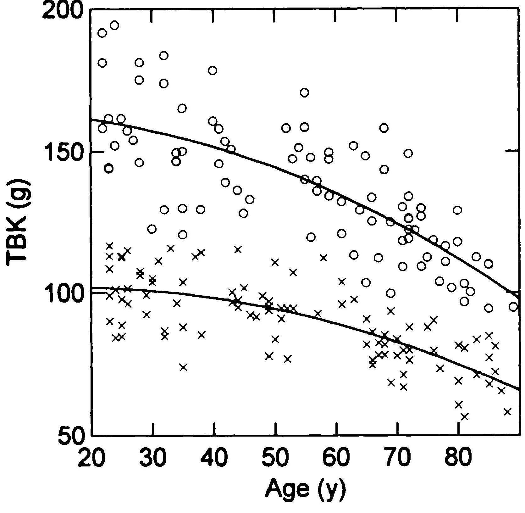

The existence of racial / ethnic dif­fer­ences in total body potas­sium has also been reported (Ellis et al., 2000). In a recent study, Shypailo and Wong (2020) presented cross-sectional data for total body potas­sium (in g) mea­sured by whole body counting by sex, race / ethnicity, for six age groups. Black children had higher amounts of total body potas­sium for certain age groups com­pared to white and Hispanic children.

The potas­sium concentration of the fat-free mass also declines with increasing obesity and during preg­nancy due to the increased hydra­tion of the fat-free mass. In obese subjects, some of the decrease may also be explained by the lower pro­por­tion of muscle in the fat-free mass and by a measure­ment error resulting from absorption of the γ‑rays by adipose tissue (Womersley et al., 1976). During preg­nancy, the potas­sium concentration of the fat-free mass is lower than for non-pregnant women (2.1g/kg vs. 2.3g/kg fat-free mass), but increases in early postpartum (Hopkinson et al., 1997).

Total body potas­sium may also be altered in clinical patients with a wasting disease such as cancer, when muscle mass is reduced (Cohn et al., 1981). Clearly, constants for the potas­sium concentration of the fat-free mass must consider age, sex, ethnicity, obesity, and preg­nancy, or estimates of fat-free mass derived from ⁴⁰K measure­ments will be in error, sometimes by as much as 20%.

The simple 2‑com­po­nent model: \[ \small \mbox { Total body fat (kg) = body weight (kg) − fat-free mass (kg) }\] allows the cal­cula­tion of total body fat (kg) from the fat-free mass (kg). However, any errors and uncer­tain­ties in the cal­cula­tion of the fat-free mass from ⁴⁰K measure­ments will be propogated into the derived cal­cula­tion of total body fat (Silva et al., 2013). These uncertain­ties can limit the applic­ation of the 2‑com­po­nent model in clinical popu­lations with certain disease states, particularly a wasting disease such as cancer, when total body potassium measurements are low as a result of loss of muscle mass. Conse­quently, in these circum­stances, use of the 2‑com­po­nent model to derive indirectly total body fat is inappropriate. Instead, more sophisticated body compo­sition models, involving 3‑ or 4‑com­po­nents, that reduce the need for under­lying assump­tions, should be used.

14.3 Total body water from isotope dilution

Either the stable isotope deuterium (²H), the radio-active isotope tritium (³H), or the stable isotope of oxygen (¹⁸O) can be used to measure total body water. Of the three, deuterium is now most frequently used. Standardized conditions are necessary for the measure­ment because fluid and food intake and exercise can all affect total body water concentrations. As a result, samples should be taken in the morning, after an overnight fast and the bladder has been emptied, and with a restriction of fluid intake.

A tracer dose of sterile water labeled with an accurately known amount of the isotope (often deuterium oxide, D₂O) is administered either orally or intravenously to the subject and allowed to equilibrate. Two samples of serum, or urine, or saliva are collected; one prior to the administration of the tracer and a second after the isotope has equilibrated with the subject's water pool (usually 3‑5h post-dose). The baseline sample measures the naturally present isotope in the total body water. The enrichment observed in the post-dose sample allows cal­cula­tion of the total body water. The measure­ment of enrichment appears to be less reliable in urine than in serum probably because of the longer equilibration period of the bladder contents relative to blood.

Ideally, no food or water is permitted during equilibration, which may take 3‑5h, depending on the isotope, the physiological sample, and the health condition of the patient. If fluid has been taken during the equilibrium period, a cor­rec­tion can be made, where necessary, to derive actual body water (Gutiérrez-Marín et al., 2019). Longer equilibration periods are necessary for urine com­pared to blood serum samples, for obese patients (Schoeller et al., 1980), or for those with edema, ascites, and shock (McMurrey et al., 1958). Table 14.2 demonstrates that the method is relatively robust and, inde­pen­dent of the dif­fer­ent physiological fluids used.

Table 14.2. A demonstration of the relatively small variations in total body water (TBW), when calculated from isotopic enrichments of dif­fer­ent physiological fluids and at dif­fer­ent times postdose.
* Ratio: TBW_A/TBW_B.
From Schoeller et al. (1985).

Samples (A) & (B)	Isotope	n	*Ratio	SD
(A) Saliva at 4h (B) Serum at 4h	18O	33	1.006	0.019
(A) Urine at 6h (B) Serum at 6h	18O	11	1.012	0.027
(A) Urine at 12h (B) Serum at12 h	18O	14	1.006	0.010
(A) Saliva at 3h (B) Saliva at 4h	18O	20	0.997	0.005
(A) Saliva at 3h (B) Saliva at 4h	2H	43	0.996	0.007

The cal­cula­tion of total body water is based on the extent to which the isotopic dose is diluted by the total body fluid as shown below: \[ \small \mbox { Total body water = (V × C) / (C}_{2} \mbox {− C}_{1}) \] where V = volume of dose, C = concen­tration of admin­istered isotope, C₁ = baseline concen­tration of isotope in serum / urine / saliva, and C₂ = concen­tration of isotope in serum / urine / saliva sample after equilibration.

A cor­rec­tion may be necessary for urinary loss of the tracer. Details of the isotope dilution methods and the limit­ations encountered when mea­sur­ing total body water in the field have been reviewed by Schoeller (1991) and Ellis (2001), respectively.

The isotopic tracer chosen and the method used for analysis are inter­related. Tritium (³H) is easy to measure with a scintillation counter but involves radiation to the subject, making the technique unsuitable for children and women of child­bearing age (Schoeller et al., 1980), and when repeated measure­ments over a short time period are necessary. The non­radio­active isotope ¹⁸O must be mea­sured by mass spectrometry. The stable isotope deuterium is now the tracer of choice because it is much cheaper than ¹⁸O and can be mea­sured by infrared absorption, gas chromatography, an isotope ratio mass spectrometer, and more recently by Fourier transform infrared spectrophotometry (FTIR). Use of FTIR for deuterium (²H) analysis is less expensive and quicker, although slightly less precise than the use of an isotope ratio mass spectrometer. Saliva is preferred to urine as the chosen body fluid when using FTIR for the measure­ment because urine may cloud the optical lens of the FTIR (Owino et al., 2017). For a comprehensive description of the use of FTIR for the analysis of deuterium in saliva, see:

https://nucleus.iaea.org/HHW/Nutrition/BodyComposition/RefsBodyComp/index. html#publ

Recently, an alternative FTIR spectroscopic method (ATR FTIR) has been developed which requires a smaller volume of plasma (10µl), and has shorter analyses times, making it suitable for use in pediatrics; for more details, see Ward (2021).

14.3.1 Application of body water measure­ments by isotope dilution

The measure­ment of total body water in both healthy and diseased persons is the most important applic­ation of isotope dilution techniques. All body water is present in the fat-free mass. Hence, total body water measure­ments can be used to estimate the fat-free mass. This estimation requires an assumed value for fat-free mass hydra­tion, as shown below: \[ \small \mbox {Fat-free mass (kg) = (total body water (kg)) / hFFM }\] where hFFM = hydra­tion of the fat-free mass.

Based on the 2‑com­po­nent model, once the fat-free mass has been deter­mined, total body fat (TBF) and per­cent­age of body fat can be calculated as shown below: \[ \small \mbox {Total body fat (kg) = body weight (kg) − fat-free mass (kg) }\] \[ \small \mbox {% body fat = (Total body fat (kg) × 100%) / body weight (kg) }\]

Table 14.3. Median values for hydra­tion by sex. Data from Wells et al. (2010) who also present data for inter­vening years.

Age	Males Hydration (%)	Females Hydration (%)
5y	76.5	76.7
7y	76.1	75.5
9y	75.7	75.1
11y	75.3	75.0
13y	75.0	74.6
15y	74.4	74.1
17y	73.7	73.7
19y	73.4	73.6

In healthy adults, hFFM is assumed to be 0.732. However, use of a single value for the hydra­tion of fat-free mass may lead to errors in derived values for the fat-free mass. For example, hFFM is known to vary during hormonal cycles in women and in certain disease states owing to under-hydra­tion. Alternatively, over-hydra­tion due to edema, may arise among children with severe acute malnutrition (Gutiérrez-Marín et al., 2019; Most et al., 2018). The hydra­tion of fat-free mass is also known to change during growth and mat­ura­tion. At birth hFFM is about 80%, after which it grad­ually decreases until reaching the adult value (Schoeller, 1989). The refer­ence values for hFFM by age and sex in children aged 5‑20y compiled by Wells et al. (2010) are shown in Table 14.3, and are similar to earlier values reported for males but about 2% lower for females in mid-childhood (Lohman, 1989).

Hydration values for the fat-free mass are also affected by obesity, the increase said to be due to an expansion of extra­cellular water, although other mechanisms may be involved (Leone et al., 2000); see Chumlea et al. (2007) for more details. Note the marked increase in hFFM (as %) in heavier BMI groups shown in Figure 14.2 based on a large study of subjects from 4‑22y (Gutiérrez-Marín et al., 2019). This same trend has been reported previously in smaller studies of obese children (Haroun et al., 2005; Wells & Fewtrell, 2006) and adults (Waki et al., 1991), and high­lights that refer­ence data for hydra­tion values for higher BMI groups are also needed to avoid bias.

Pregnancy is also associ­ated with an increase in hFFM, as noted in Section 14.2. Published values for hFFM at specific time points in preg­nancy are shown in Figure 14.3.

The equa­tions of van Raaij et al. (1988), based on ten-week inter­vals through­out gestation, are those most used in 2‑com­po­nent models to estimate maternal fat mass during preg­nancy. A regression equa­tion based on the van Raaij et al. (1988) data has been developed allowing estimation of hFMM for any given time throughout gestation; this regression line is also shown in Figure 14.3.

Table 14.4. Effect of adopting dif­fer­ent hydra­tion constants on fat mass (FM) and fat-free mass (FFM) calculated at 30 weeks gestation on women of normal weight (76kg) and total body water (45.0L). Data from Most et al. (2018).

Author	Hydration constant	FFM (kg)	FM (kg)	FM (%)
Siri (1961)	0.724	62.2	13.8	18.2
Van Raaj et al. (1988)	0.740	60.8	15.2	20.0
Fidanza (1987).	0.752	59.8	16.2	21.3
Catalano et al. (1995)	0.762	59.1	16.9	22.3

Table 14.4 high­lights the effect of adopting dif­fer­ent hydra­tion constants on the assess­ment of fat-free mass and fat mass in a women at 30wks gestation with a normal pre-gravid BMI (i.e., 24.8kg/m²). Clearly, failure to consider the increase in hFFM in models based on total body water using isotope dilution would result in an overestimate of the actual fat-free mass in pregnant women, and thus under­estimate fat mass when the 2‑com­po­nent model is applied.

Recently, refer­ence charts for infants and children aged from 6wks to 5y by sex have been developed for per­cen­tiles for total body water mea­sured by deuterium dilution, and fat-free mass calculated from total body water using pub­lished hydra­tion coefficients (Wells et al., 2020). These charts will help clinicians identify how specific diseases and their treatment impact on fat-free mass and fat mass in this age group.

The error associ­ated with the measure­ment of total body water using these isotopic tracers is typically less than 1kg. This error equates to an uncertainty of about 10% (about 1.4kg) in the absolute fat mass of an average healthy adult or 2% in the estimate of per­cent­age of fat. These relatively low errors have resulted in the isotope dilution method becoming the refer­ence or gold-stan­dard method in com­par­ison with other measure­ment pro­ce­dures for total body water (e.g., bio­elec­trical imped­ance: Section 14.8).

A 3‑com­po­nent model that partitions body weight into three major com­po­nents can also be used to measure fat-free mass and fat mass: \[ \small \mbox { Body mass = fat + water + residual }\] where residual (i.e., fat-free dry mass) is the sum of protein, bone mineral, and glycogen

This 3‑com­po­nent model partitions the body mass into fat, total body water, and the remaining fat-free dry mass, which is assumed to have a constant ratio of protein to mineral. This 3‑com­po­nent model avoids the assump­tion that the water content of fat-free mass is the same for all indi­viduals of a given age and sex. Instead, the model provides an estimate of the hydra­tion and density of fat-free mass. Three measure­ments are made: body weight (in kg), body volume (in liters), and total body water (in liters). Fat mass can be calculated from these three basic measure­ments by applying the 3‑com­po­nent model of Siri (1961) which includes both whole body density and total body water; see Wells et al. (1999) and Fuller et al. (1992) for further details. This version of the 3‑com­po­nent model provides improved practical estimates of both the fat mass and fat-free mass in children (Silva et al., 2013).

14.4 Multiple dilution methods

Multiple dilution can be used to estimate the volume of various body fluid com­part­ments that, in turn, can be used to estimate two com­po­nents of the fat-free mass: extra­cellular mass (ECM) and the body-cell mass (BCM).

Typically, multiple dilution involves determining both total body water (via isotope dilution; Section 14.3) and extra­cell­ular water (ECW), the latter using a tracer such as bromide that does not enter the intra­cell­ular space (Wong et al., 1989). The dif­fer­ence between these two measure­ments (i.e., TBW − ECW) reflects the intra­cell­ular water (ICW), which is more metabolically active than ECW and provides an estimate of BCM (Ribeiro & Kehayias, 2014).

To estimate BCM using this approach, a pre-dose blood or urine sample is taken followed by dosing with deuterium oxide and sodium bromide solution. After a 3‑5h equilibration period, a final post-dose blood or urine sample is collected, although longer equilibration periods are needed for indi­viduals with expanded ECW, including those with extreme obesity. Deuterium enrichment of the bio­logical sample is described in Section 14.3, whereas bromide enrichment is deter­mined by high-per­form­ance liquid chromatography or non-destructive liquid X‑ray fluorescence. The reported precision for ICW calculated using this approach is about 2.5% provided stan­dardized protocols are used (Earthman, 2015). The ratio of ECW / TBW can also be calculated using this approach. In a study of nursing home elderly, the ratio ECW / TBW was signif­icantly higher com­pared to the ratio in free-living elderly, prompting the sug­ges­tion that this ratio may have potential as a surrogate method for the clinical assess­ment of frailty (Kehayias et al., 2012).

14.4.1 Application of multiple dilution methods

The ECM is defined as the com­po­nent of the fat-free mass which exists outside the cells. It consists of both fluid (e.g., extra­cellular fluids, plasma volume) and solid (e.g., skeleton, cartilage, tendons) com­po­nents which are involved in transport and support and are not metabolically active.

In contrast, the BCM is the total mass of cells in the body that consume oxygen and produce work (i.e., the metabolically active, energy-exchanging mass of the body). These com­po­nents are the nonfat cellular portion of tissues, primary the skeletal muscle, organ tissue mass, blood, and the brain (Wang et al., 2004). Nutritional status, physical activity level, and disease states alter BCM, which thus serves as a helpful bio­marker.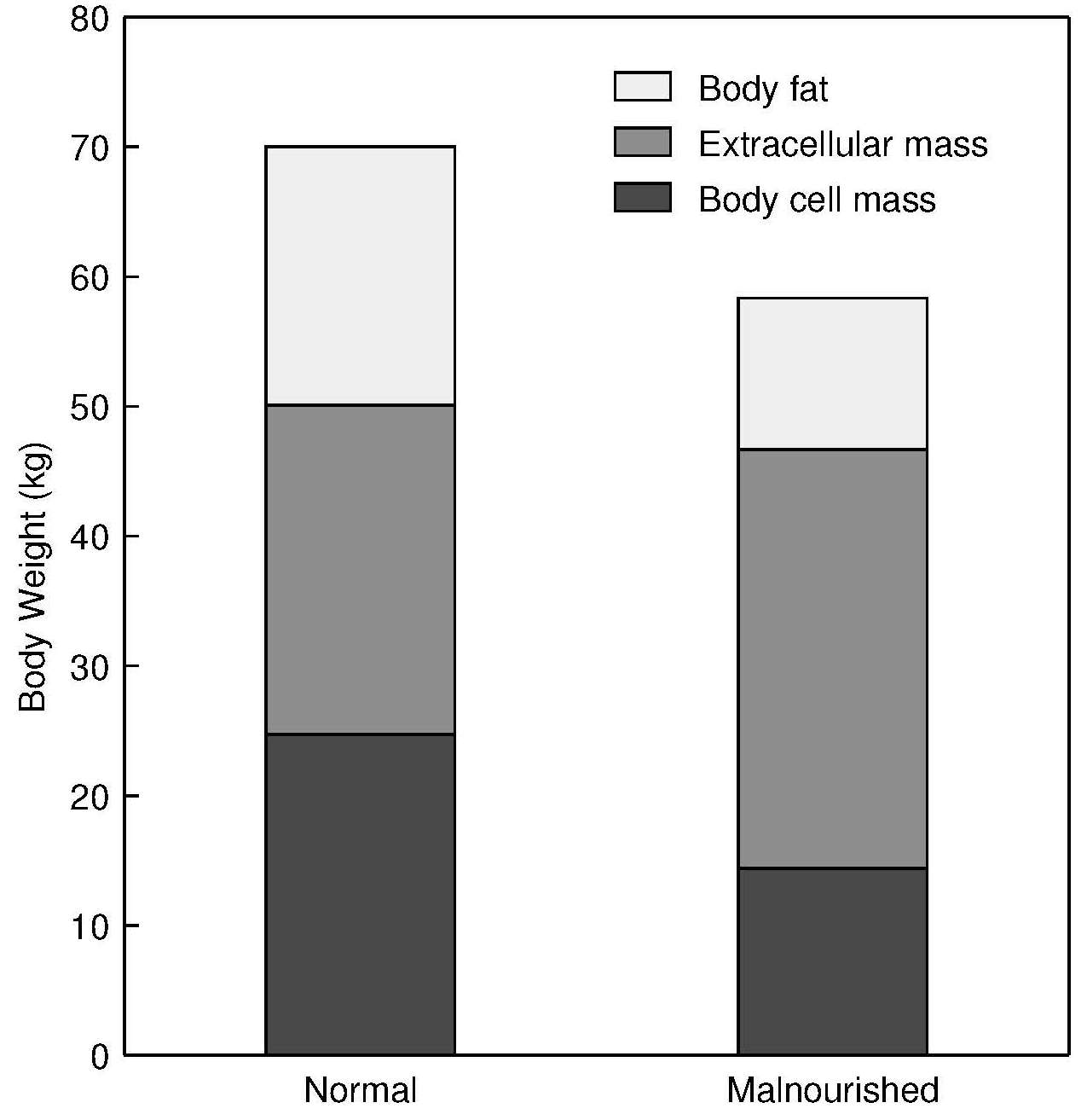

Measure­ments of BCM and ECM are especially critical in mal­nour­ished patients. Values for total fat-free mass in these patients may remain unchanged, but the compo­sition of the fat-free mass is abnormal, with a reduced BCM, concomitant with an expansion of the ECM, as shown in Figure 14.4. Hence, any loss in body weight in such patients reflects a loss of body fat (Shizgal, 1987).

14.5 In vivo activ­ation analysis

A group of related techniques involving in vivo neutron activ­ation analysis (NAA) allow the direct estimation of the amount of a range of chemical elements in the living human body. Most other techniques used in body compo­sition studies, with the exception of whole body counting for potas­sium, gen­er­ate data on tissue density or volume, but not data on the amount of a com­po­nent. As a result, multicom­po­nent elemental models based on in vivo NAA have grad­ually become accepted as refer­ence methods for the cali­bra­tion of many of the other techniques described in this chapter.

Nearly all the major elements present in the body can be analyzed by in vivo NAA, including hydrogen, oxygen, carbon, nitrogen, calcium, phosphorus, sodium, and chlorine (Cohn et al., 1984). Of special inter­est is the applic­ation of NAA to measure the carbon-to-oxygen (C/O) ratio in vivo . This ratio can provide an inde­pen­dent, unbiased measure of the distribution of fat and fat-free mass, which is not dependent on the assump­tions about the compo­sition of fat-free mass. Small changes in fat-free mass can be monitored, making the method appropriate for studying the depletion of fat-free mass with aging (Kehayias et al., 2000).

A major negative factor associ­ated with in vivo NAA is that the subject is exposed to radiation. This and the associ­ated risks must always be explained to the subject. In vivo NAA is most used in clinical medicine for the deter­min­ation of total body nitrogen (TBN), total body calcium (TBCa), and bone mass as discussed below. TBN and TBCa are only deter­mined in a relatively small number of laboratories worldwide — an indication of the expense involved and tech­nical difficulties associ­ated with the method.

14.5.1 Total body nitrogen by in vivo NAA

Nitrogen is normally deter­mined by NAA by bombarding the patient, in a supine position, with a low neutron flux from a ²³⁸PuBe source or from a cyclotron or neutron generator. During irradiation, a pro­por­tion of ¹⁴N is converted to an excited state of ¹⁵N, which decays almost immediately to its ground state, emitting a “prompt” γ‑ray at 10.83MeV. This activity is counted by an array of sodium iodide detectors in a whole body counter (Figure 14.5).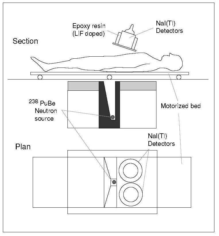

The detected γ‑ray counts are pro­por­tional to the absolute mass of total body nitrogen (Beddoe & Hill, 1985). Measure­ment of the nitrogen content of the body gives a measure of total body protein because the mass of nitrogen bears a fixed ratio to the mass of protein (1g N = 6.25g protein). The radiation expo­sure using this method is about 0.3mSv. This compares with the national back­ground radiation from cosmic and other sources of about 3.5mSv/y.

The 10.83MeV γ‑ray is specific to nitrogen and is at an energy which is not affected by inter­ference from other reactions. Extensive shielding, how­ever, is necessary around the sodium iodide detectors to reduce the level of back­ground radiation. Never­the­less, cor­rec­tions to the γ‑count must still be made for the back­ground.

The cali­bra­tion of the counter is critical and must consider the height, weight, and adiposity of the subject because of the varying neutron attenuation and internal absorption of the emitted γ‑rays. Calibration is achieved using phantoms or by using hydrogen as an internal stan­dard Vartsky et al., 1979).

The accuracy of prompt γ‑neutron activ­ation for mea­sur­ing total body nitrogen has been validated by comparing total body nitrogen in two human cadavers with results obtained by direct chemical analysis of nitrogen (Knight et al., 1986). Close agreement between the two techniques was found. This study also confirmed the use of the ratio 6.25 for the relation­ship between total body protein and total body nitrogen.

14.5.2 Application of body nitrogen by in vivo NAA

Changes in total body protein of hospital patients with diseases such as cancer, renal dysfunction, hypertension, chronic heart disease, and rheumatoid arthritis, and with severe trauma or sepsis have been studied using prompt γ‑neutron activ­ation (Beddoe & Hill, 1985). The results indicate that sub­stantial losses of body protein may occur, even when conven­tionally adequate nutritional support has been provided for some of these patients. Depleted total body protein is also a consistent finding among acutely ill anorexic patients. In a longitudinal study, Haas et al. (2018) reported that after recovering from anorexia nervosa, depletion of body protein mea­sured by in vivo INAA remained in adolescent patients after 7mos, even though body weight was restored. Clearly, further work is required to identify nutritional inter­vention pro­ce­dures which minimize loss of body protein in hospital patients and those with anorexia nervosa.

14.5.3 Total body calcium by in vivo NAA

The method is based on the conversion of a pro­por­tion of the naturally occurring isotope ⁴⁸Ca in the body to ⁴⁹Ca (half-life = 8.8min) by exposing the patient to a low neutron flux. Immediately following irradiation, the patient is transferred to a whole-body counter, and the γ‑rays emitted by the decay of ⁴⁹Ca are detected by an array of sodium iodide detectors.

The counting geometry is similar to that used for total body potas­sium, and again care must be taken in positioning the subject and correctly accounting for the varying height, weight, sex, and body mass index of subjects. In particular, for subjects with BMI > 30, the effects of neutron attenuation become signif­icant, necessitating additional cor­rec­tions or a special cali­bra­tion (Ma et al., 2000). The reported accuracy and precision are from 1‑2% (Cohn et al., 1974).

14.5.4 Application of total body calcium by in vivo NAA

The radiation expo­sure using this method varies from 2.5‑25mSv, depending on the neutron source. This range is considerably higher than that experienced during dual X‑ray absorp­tiometry (DXA) and limits the general applicability of the method. Conse­quently, the use of neutron activ­ation analyses for the assess­ment of total body calcium has largely been replaced by DXA (Section 14.11). Instead, the method is now mainly used as a cali­bra­tion tool for other techniques.

The assess­ment of total body calcium by in vivo neutron activ­ation analysis is also discussed in Chapter 23 under the assess­ment of calcium status.

14.6 Densitometry

Body density was one of the first measures of body compo­sition to be made Behnke et al., 1942). It is relatively easy to measure, and in the past, body density was the gold-stan­dard method to determine per­cent­age body fat using the 2‑com­po­nent model. Certain disease states characterized by excess fluid retention and under-mineralization decrease the density of fat-free mass. Conse­quently, densit­ometry is now often combined with other measures in a 4‑com­po­nent model of body compo­sition so that hydra­tion and density of fat-free mass are mea­sured along with the actual bone mineral content, thus providing a more accurate assess­ment. (Silva er al., 2013).

Hydrostatic weighing was the initial densitometric method used to determine body volume, and hence whole body density. However, it is now being replaced by plethysmo­graphic methods that are more acceptable to subjects, particularly children (Fields & Goran, 2000; Wells & Fewtrell, 2006). All three methods are described below. A concluding section describes the cal­cula­tion of body fat from body density (Section 14.6.4).

14.6.1 Hydrostatic weighing

The conven­tional method of directly mea­sur­ing whole body density involves weighing the subject and then using Archimedes' principle to determine the volume of the subject. Thus, the subject is weighed first in air and then when completely submerged in water in a large tank. The subject is instructed to squeeze out any air bubbles trapped inside the bathing suit, and to expel as much air as possible from the lungs before immersion. The hydro­static weight is recorded at the end of the forced expiration. Multiple readings should be taken using a con­tin­uous and sen­sit­ive recording of under­water mass, the heaviest corre­sponding to the most complete expiration. This method requires a high degree of water con­fid­ence and thus the method is not suitable for children younger than 8y, the elderly, obese, or unhealthy persons.

The body volume is then calculated from the apparent loss of weight in water (i.e., the dif­fer­ence between the weight of the person in air and his or her corre­sponding weight in water). Once total body mass and body volume have been deter­mined, whole body density can be readily calculated, on the basis that density is mass per unit volume and the density of water is l.0kg/L at 4°C: \[ \small \mbox { Whole body density = (body weight in air (kg)) / (apparent loss in weight (kg)) }\] Three cor­rec­tions must be applied:

• Hydrostatic weighing is usually performed in water at 30°C instead of 4°C. At this higher temperature, the density of water is 0.9957kg/L, and a water temperature cor­rec­tion factor must be applied.
• Air trapped in the lungs also contributes to the amount of water displaced by the subject under water. Residual air in the lungs can be mea­sured while the subject is in the tank. Alternatively, the volume can be estimated using a nitrogen washout, helium dilution, or oxygen dilution (Brodie, 1988). This cor­rec­tion can also be estimated from empirical equa­tions. The residual air volume is then sub­tracted from the body volume.
• The volume of the air trapped in the gastrointestinal tract also contributes to the total amount of water displaced. This volume is small and is never mea­sured. It is often taken as 100mL.

The within-subject variability in gastrointestinal gas volume, how­ever, can be quite large (0‑500mL in adults), reducing the precision of the method. Even when the above cor­rec­tions are carefully applied, considerable uncertainty remains. If the whole body density is used to calculate the per­cent­age of body fat (see below), these uncer­tain­ties become errors in the per­cent­age of body fat. The errors may be systematic rather than random in nature and may be large when the residual air volume is estimated. If the residual air volume is in error by 300‑500mL, there will be a corre­sponding uncertainty in the per­cent­age of body fat from 3‑5%.

Hydro­static weighing can give very reproducible results for whole body density, provided that the examiners and the subjects are well trained. For example, Durnin and Rahaman (1967) reported a stan­dard deviation of 0.008kg/L for serial measure­ments on three subjects over a 1y period.

14.6.2 Water-displace­ment pleth­ysmog­raphy

The use of a plethysmo­graph eliminates the necessity for totally immersing the subject in water, a disadvantage of hydro­static weighing (Section 14.6.1). For the measure­ment, the plethysmo­graph is zeroed and filled with water (Figure 14.6).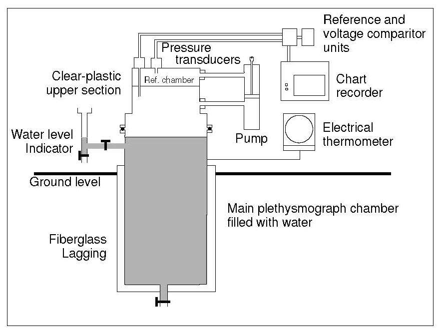

The subject is then weighed, and a weight of water equal to the weight of the subject is removed from the plethysmo­graph. The subject then stands with water up to the neck only, and the head is covered by a clear-plastic dome. The volume of air surrounding the head of the subject, and in the lungs and gut, is then deter­mined by mea­sur­ing the pressure changes produced by a pump of known stroke volume (Garrow et al., 1979). This allows the total volume of the subject to be deter­mined. The total time for the test, including three measure­ments on each subject, is about 20min.

The method has been used successfully to measure body density of obese adults (Garrow et al., 1979). Estimates of body fatness obtained com­pared favorably with those based on total body potas­sium.

Water-displace­ment pleth­ysmog­raphy has now been replaced by air-displace­ment pleth­ysmog­raphy (discussed below) for the measure­ment of total body volume. Never­the­less, water-displace­ment pleth­ysmog­raphy has been adapted to measure leg volume, and is used by clinicians to study chronic venous insufficiency (CVI). For a review of the clinical use of water displace­ment leg volumetry and the potential errors that may occur, see Rabe et al. (2010).

14.6.3 Air-displace­ment pleth­ysmog­raphy

The measure­ment of body volume has been signif­icantly eased by the development of an air-displace­ment pleth­ysmog­raphy device (Bod Pod). These devices determine the volume of a subject indirectly by mea­sur­ing the volume of air displaced by the subject inside an enclosed chamber — plethysmo­graph or Bod Pod. The method is quick, comfortable, automated, non-invasive, safe, and does not require extensive tech­nical training. For infants up to about 6mos of age, a device known as the “Pea Pod” is avail­able and can accommodate infants up to about 8kg. For small children from 2‑6y, the Bod Pod with a Pediatric Option can be used, whereas the stan­dard Bod Pod can be used for older children (i.e., > 6y), adults, and the elderly.

The air-displace­ment plethysmo­graph consists of an ovoid fiberglass structure divided into two sections: a rear refer­ence chamber and a front test chamber containing the seated subject (Figure 14.7).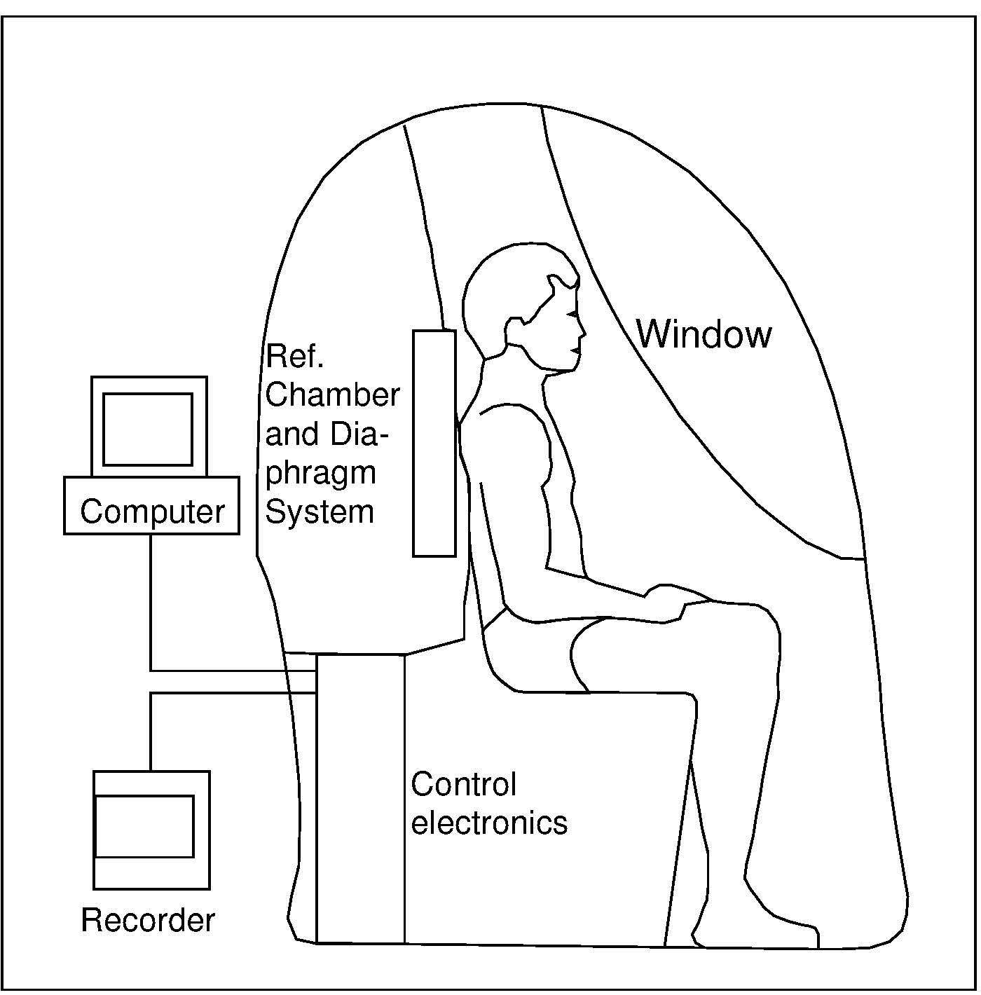

The dividing wall between the two chambers encompasses a large diaphragm. This can be made to oscillate under computer control, gener­ating com­ple­men­tary pressure changes in the test and refer­ence chambers which are recorded. These changes and the applic­ation of the basic gas laws allows the volume of the test chamber to be calculated. Measure­ments both with and without a seated subject provide infor­mation on the total body volume of the subject.

While they are seated in the test chamber, subjects should wear minimal clothing, often a swimsuit and a tightly fitting bathing cap to minimize the volume of air contained near the hair or skin, and in clothing. Measure­ments over a 1‑min period usually suffice, and an average of two separate trials should be used to calculate body volume. For details on the methods and per­form­ance of the PEA POD system for mea­sur­ing body compo­sition in infants, see Ellis et al. (2007); for moderately premature infants, see Forsum et al. (2016), and for children aged 2‑6y, see Fields et al. (2012).

A cor­rec­tion for the average volume of air in the lungs and thorax during normal breathing (VTG) should be applied. This can be mea­sured while the subject is in the test chamber (Dempster & Aitkens, 1995), or predicted based on age, sex, and height (McCrory et al., 1998). Pregnancy must also be considered because thoracic gas volume declines throughout preg­nancy by about 100mL per trimester. Hence, VTG needs to be adjusted for the trimester-specific decline in lung volume (Most et al., 2018). Once body volume has been mea­sured, whole body density (D) can be calculated from mea­sured body mass.

For a com­par­ison of the com­po­nents and capabilities of the three pleth­ysmog­raphy techniques, see Fields et al. (2015).

14.6.4 Application of densit­ometry to calculate body fat

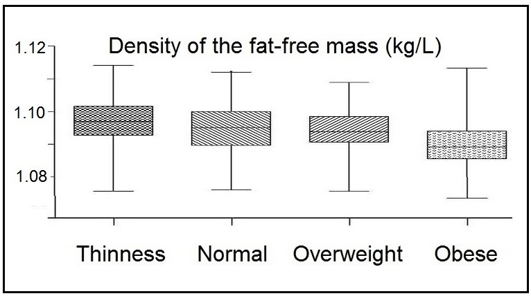
Once whole-body density has been mea­sured by one of the methods outlined above, the per­cent­age body fat can be calculated. This involves the selection of an empir­ical densito­metric equa­tion relating fat content to whole body density (D). Several empir­ical densito­metric equa­tions have been derived based on the classic two-com­po­nent model for body compo­sition. As noted earlier, in this model body weight is divided into fat and fat-free mass, and relies on assump­tions that ignore inter-indi­vidual variability in the compo­sition of the fat-free mass.

All the classical densitometric equa­tions shown below assume:

• The density of the fat-free mass is relatively constant.
• The density of fat for normal persons does not vary among indi­viduals.
• The water content of the fat-free mass is constant.
• The pro­por­tion of bone mineral (i.e., skeleton) to muscle in the fat-free body is constant.

The dif­fer­ent authors all assume the density of fat and the fat-free mass do not change with age and sex. There are two constants in each equa­tion, C₁ and C₂, the dif­fer­ent authors suggesting slightly dif­fer­ent values for each: \[ \small \mbox { %F = ((4.950/D) − 4.500) × 100% (Eq.A) }\] \[ \small \mbox { %F = ((4.570*/D) − 4.142) × 100% (Eq.B) }\] \[ \small \mbox { %F = ((5.548*/D) − 5.044) × 100% (Eq.C) }\] The Siri (1961) equa­tion (Eq.A) is most widely used and assumes that the densities of fat and fat-free mass are about 0.90 and 1.10kg/L respectively. Brožek et al. (1963) (Eq.B) and Rathbun and Pace 1945) (Eq.C) used the concept of a refer­ence man of a specified density and compo­sition; these equa­tions avoid the requirement of esti­mat­;ing the density of fat-free mass. The constants applied in all these equa­tions came from the chemical analysis of a few adult cadavers dissec­tions, animal data, and indirect estimates of fat-free mass in human subjects (Heymsfield et al., 1991; Silva et al., 2013).

None of these classical empirical equa­tions relating fat content to body density, how­ever, are suitable for adult patients in clinical settings when the compo­sition of their fat-free mass may be abnormal. This will include patients under­going hyper­alimentation with high-sodium fluids, or with congestive heart failure or liver disease, as total body water content as a fraction of fat-free mass may be markedly higher in these patients, thus violating the assump­tion that the water content of the fat-free mass is a constant (i.e., 73.2%). In these patients, the density of fat-free mass is decreased. Not surprisingly, in patients with diseases associ­ated with under-mineralization, the density of fat-free mass is also decreased (Werdein & Kyle, 1960). Conse­quently, in all these patients, fatness will be overestimated when the 2‑com­po­nent model is applied (Wells & Fewtrell, 2006). More recent research has raised concerns over the assump­tion of constant properties for hydra­tion and density of fat-free mass when these classical empirical equa­tions are applied to assess body compo­sition not only in patients with certain diseases, but also in healthy children and adolescents, the elderly, pregnant women and those with obesity, as noted earlier.

Although fat has relatively uniform properties throughout the life course (zero water and a density of 0.9007kg/L), in contrast fat-free mass has dif­fer­ent properties in children com­pared to adults. This arises because of chemical mat­ura­tion of the fat-free mass during growth which results in higher levels of water and lower levels of mineral and proteins, and thus changes in the hydra­tion and density of the fat-free mass (Wells et al., 2010), as noted earlier. Never­the­less, the adult-derived values for the density and hydra­tion of fat-free mass and applied in the classical equa­tions shown above have often been used to study body compo­sition in children (Silva et al., 2013).

In an effort to improve the accuracy in the estimates of per­cent­age body fat based on pediatric densit­ometry (and hydro­metry, Section 14.3, Wells and co-workers mea­sured body compo­sition via a 4‑com­po­nent model in a large, healthy sample of children and adolescents aged 4‑23y. Use of this model overcomes the limit­ations associ­ated with the assump­tions of constant properties for hydra­tion and density of fat-free mass applied in the Siri equa­tion.

Table 14.5. Median values for hydra­tion, density, and constants (C₁ and C₂) for the pediatric version of the equa­tion of Siri (1961), obtained by using the LMS (lambda, mu, sigma) method. Data from Wells et al. (2010).

	Males				Females
Age	Hydra- tion (%)	Density (kg/L)	C1	C2	Hydra- tion (%)	Density (kg/L)	C1	C2
5y	76.5	1.0827	5.36	4.95	76.7	1.0837	5.33	4.92
6y	76.3	1.0844	5.32	4.90	76.1	1.0865	5.27	4.85
7y	76.1	1.0861	5.28	4.86	75.5	1.0887	5.22	4.79
8y	75.9	1.0877	5.24	4.82	75.2	1.0900	5.19	4.76
9y	75.7	1.0889	5.21	4.79	75.1	1.0909	5.17	4.74
10y	75.5	1.0900	5.19	4.76	75.0	1.0916	5.15	4.72
11y	75.3	1.0911	5.16	4.73	75.0	1.0924	5.13	4.70
12y	75.2	1.0917	5.15	4.72	74.9	1.0937	5.10	4.67
13y	75.0	1.0920	5.14	4.71	74.6	1.0954	5.07	4.63
14y	74.8	1.0927	5.13	4.69	74.4	1.0975	5.02	4.58
15y	74.4	1.0942	5.09	4.66	74.1	1.0996	4.98	4.53
16y	74.0	1.0960	5.05	4.61	73.8	1.1011	4.95	4.49
17y	73.7	1.0978	5.02	4.57	73.7	1.1020	4.93	4.47
18y	73.5	1.0991	4.99	4.54	73.6	1.1027	4.92	4.46
19y	73.4	1.1000	4.97	4.52	73.6	1.1031	4.91	4.45
20y	73.3	1.1006	4.96	4.51	73.6	1.1035	4.90	4.44

Their results confirmed that the previously pub­lished adult values for the density and hydra­tion of fat-free mass when applied to pediatric popu­lations were inappropriate. They developed new empirical age‑ and sex-specific refer­ence values for the hydra­tion and density of fat-free mass; these are shown in Table 14.5. In addition, they developed pre­dic­tion equa­tions of density and hydra­tion for fat-free mass by age, sex, and body mass index (BMI) SD score; see Wells et al. (2010) for more details.

Note that the values for the C₁ and C₂ constants for the adult males (age 20y), shown in Table 14.5, are similar to the corre­sponding values shown in the Siri equa­tion above (i.e., 4.95 for C₁ and 4.50 for C₂), whereas for adult females, the corre­sponding values are slightly lower: 4.90 for C₁ and 4.44 for C₂ at 20y. With the substitution of the age- and sex-specific C₁ and C₂ constants from Table 14.5 in place of the C₁ (4.95) and C₂ (4.50) constants in the Siri equa­tion, the accuracy of the 2‑com­po­nent model for esti­mat­ing fat mass of a healthy pediatric popu­lation based on densit­ometry could be improved.

More recent research has high­lighted increasing values for hydra­tion of fat-free mass (see Section 14.3 and Figure 14.3) but decreasing values for the density of fat-free mass in the children with a heavier body mass index (BMI) (Figure 14.8). This trend was observed earlier in children (Haroun et al., 2005) and adults (Waki et al., 1991). Gutiérrez-Marin et al. (2021) have developed a predictive equa­tion to estimate the density of fat-free mass for use when using a 2‑com­po­nent model to assess children and adolescents with dif­fer­ent degrees of obesity. Application of the equa­tion shown below improves the accuracy and precision of the density of the fat-free mass (DFFM) estimates in this popu­lation. \[ \small \mbox { DFFM = 1.0791 + (0.009 × age + 0.0021 × gender) − (0.0014 × BMISDS) }\] Where age is in years; gender 1 (male), 2 (female); DFFM = density fat-free mass; BMISDS = body mass index Z‑score

An excel file with all the steps in the cal­cula­tion is avail­able online as supplementary material in Gutiérrez-Marin et al. (2021).

Similar trends in the values for the hydra­tion and density of fat-free mass have been observed in studies of older Hispanic Americans (González-Arellanes et al., 2019) and obese Mexicans (González-Arellanes et al., 2021) all aged > 60y. Again values for fat-free mass density were lower, but higher for the hydra­tion fraction suggesting that modifying the assump­tions regarding both the density and hydra­tion values for fat-free mass applied in the classical densitometric empirical equa­tions may also be appropriate for the elderly and in conditions of obesity. Once per­cent­age body fat has been calculated, then total body fat (TBF) and/or fat-free mass can be derived as follows: \[ \small \mbox { Total body fat (kg) = body wt (kg) × % body fat ÷ 100 }\] \[ \small \mbox { Fat-free mass (kg) = body wt (kg) − total body fat (kg). }\]

14.7 Total body elec­trical conduc­tivity

Total body elec­trical conduc­tivity (TOBEC) is mea­sured by observing the changes induced by placing the subject in an electromagnetic field Baumgartner, 1996). The extent of the change depends on the overall elec­trical conduc­tivity of the body and, in particular, on the pro­por­tions of fat and the fat-free mass in the body: the fat-free mass, comprised largely of water with dissolved electrolytes, will readily conduct an applied electric current, whereas fat is anhydrous and a poor conductor. In more modern equipment, the subject lies supine on a motor­ized bed (Figure 14.9) that is passed in a series of steps progressively through a uniform solenoid coil.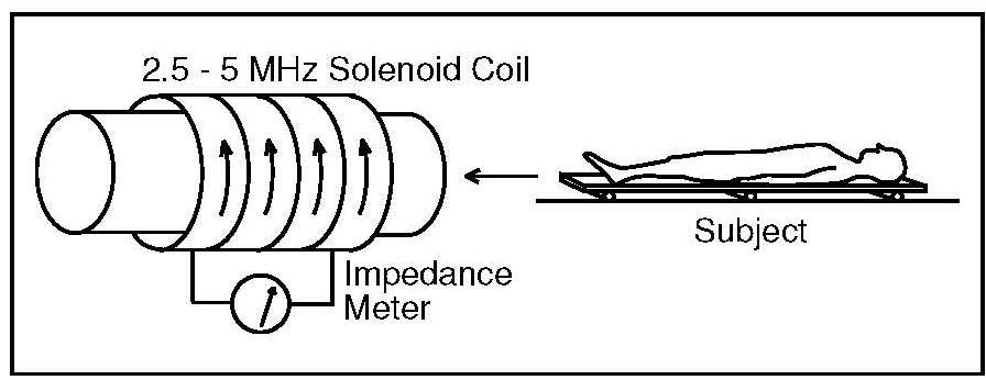

A 2.5MHz oscillating radio­fre­quency current is passed through the coil. This induces an electro­magnetic field in the space enclosed by the coil, which, in turn, induces a current in the subject, the magni­tude depending on the conduc­tivity of the subject. A second reading is taken when the coil is empty; the dif­fer­ence represents the measure­ment. The use of Fourier analysis improves the assess­ment of the lean body mass (Van Loan & Koehler, 1990).

Measure­ment of TOBEC is simple, safe, non­invasive, fast, and causes no dis­com­fort to the subjects. The tech­nique can be used on indi­viduals who cannot be weighed under­water. However, the instrument is expensive.

Careful consideration must be given to the positioning of the subject and cor­rec­tions for body geometry and length applied. Treuth et al. (2001) used a variety of techniques, including TOBEC, to determine body compo­sition in 8y pre­pubertal girls. The authors concluded that the deter­min­ations are highly method dependent and that results from all six methods studied (TOBEC, total body potas­sium, isotope dilution for total body water, bio­elec­trical imped­ance, anthropometry, and DXA) are not inter­changeable. The results high­light how TOBEC measure­ments can be evaluated by com­par­ison with other methods. Unfortunately, most of the other methods are also subject to error and bias.

14.7.1 Applications of total body elec­trical conduc­tivity

To inter­pret TOBEC measure­ments in terms of the quantity of fat-free mass in the body, a cali­bra­tion equa­tion is applied gen­er­ated by mea­sur­ing the fat-free mass of a refer­ence popu­lation using an alternative technique and relating this to the TOBEC value of each indi­vidual. A cali­bra­tion equa­tion has also been developed to measure fat-free mass and fat reliably and precisely in neonates through 1y of age (Fiorotto & Klish, 1991; Fiorotto et al., 1995).

TOBEC is relatively insen­sit­ive to shifts of fluid or electrolytes between the intra­cellular and the extra­cellular com­part­ments and to variations in bone mineral­ization. For example, in a study of middle aged and elderly subjects (35‑90y), higher values for fat-free mass were reported when predicted from measure­ments based on TOBEC com­pared to those for fat-free mass predicted by using densit­ometry or hydrometry (Van Loan & Koehler, 1990). These find­ings led to the sug­ges­tion that the higher fat-free mass values arise because the TOBEC signal is unaffected by decreases in bone mineral­ization.

14.8 Bioelec­trical imped­ance

The use of bio­elec­trical imped­ance (BIA) for the assess­ment of body compo­sition is wide­spread, in large part due to the affordability, porta­bility, and ease of use of the bio­impe­dance devices. None of the BIA devices measure body compo­sition directly. They measure an elec­trical response of the body, resis­tance, when exposed to an elec­trical current. The resis­tance mea­sured is transformed into a pre­dic­tion of total body water by an algorithm, and from that the body fat mass is deter­mined.

Three categories of BIA devices are avail­able commercially: single-fre­quency (SF‑BIA), multiple-fre­quency (MF‑BIA), and bio­impe­dance spec­tros­copy (BIS); these are described below together with some new developments in BIA. Both the SF‑BIA and MF‑BIA devices rely upon popu­lation-specific pre­dic­tion equa­tions. In contrast, BIS uses bio­physical modeling to estimate body com­part­ments. All the algorithms are based on or validated against other body compo­sition refer­ence methods, which are not totally accurate and error-free. Each BIA device works with an inbuilt algorithm specific to the device and for the popu­lation for which the algorithm was developed so it is not possible to compare studies unless the same combination of device / equa­tion / popu­lation is used (Ward, 2019; Sheean et al., 2020). Furthermore, the refer­ence popu­lation on which the BIA algorithm was based must be appropriate for the target subject being mea­sured (Lemos & Gallagher, 2017).

Many factors may influence the precision and accuracy of BIA techniques. They include factors associ­ated both with the indi­vidual (e.g., degree of adiposity, fluid and electrolyte status, skin temperature) and with the environment (ambient temperature, proximity to metal surfaces and electronic devices), the assump­tions under­lying pre­dic­tion or modeling equa­tions, instrumentation, and variations in the protocols used for the BIA measure­ments. Box 14.2 presents recommendations for optimizing whole body BIA measure­ments. The level of precision produced by both SF‑BIA and MF‑BIA devices is said to be good, with variability between repeat measures reported as 1%‑2%. For BIS measure­ments, precision is more variable (i.e., 2%‑3%) (Earthman, 2015).

In general, many BIA devices yield relatively valid estimates of fat-free mass and other body com­part­ments in healthy normal-weight indi­viduals and for large-scale epidemiological studies (i.e., mean level accuracy), but results in clinical settings, especially for indi­viduals with fluid overload, have been mixed. None of the devices gen­er­ate valid estimates for whole body compo­sition in indi­viduals with obesity (Earthman, 2015).

Like TOBEC (Section 14.7), BIA also depends on the dif­fer­ences in elec­trical conduc­tivity of a weak alternating current which flows at various rates depending on the compo­sition of the body. The current is well conducted by tissues with a high water and electrolyte content such as blood and skeletal muscle but is poorly conducted by adipose tissue, bone, and air-filled spaces which have a low water and electrolyte content. The voltage decrease of the current as it passes through the body is detected through current sensing surface elec­trodes, and the imped­ance data are recorded by the BIA device. See Kyle et al. (2004) for details of the theory of BIA.

The placement of the adhesive elec­trodes to the body is important and varies, depending on the device and whether whole-body or segmental measure­ments are sought. The stan­dard placement is a wrist-ankle tetrapolar arrangement on the hand and foot of one side of the body. Alternatively, the elec­trodes can be placed on both sides of the body on both limbs using an 8-electrode arrangement, or on dif­fer­ent segments of the body. For the stand-on BIA devices, direct contact with the elec­trodes is achieved at the feet and/or hands depending on the device.

The extrapolation from raw imped­ance data to volume depends on several key assump­tions. For example, one of the assump­tions is that stature is an acceptable surrogate for the unknown true length of the conductor, whereas another assumes the human body is comprised of five cylinders of uniform cross-sectional area. Unfortunately, these assump­tions are often violated, especially those related to body dif­fer­ences in geometry in indi­viduals with obesity and/or longer or shorter than average limbs. With the introduction of segmental and MF‑BIA techniques, some of the limit­ations of the BIA method for these indi­viduals have been overcome. For patients with clinical conditions in which hydra­tion is altered (e.g., heart or liver failure), how­ever, assuming a fixed hydra­tion will yield body compo­sition estimates that are inaccurate. For a detailed description of the assump­tions, see Mulasi et al. (2015).

14.8.1 Single-fre­quency bio­elec­trical imped­ance (SF‑BIA)

Single fre­quency BIA devices (SF‑BIA) were the earliest devices developed. With these, the imped­ance of a weak elec­trical current (typically 500‑800mA) and a single current fre­quency (i.e., typically 50kHz) is passed between two elec­trodes, usually located in the stan­dard wrist-ankle tetrapolar arrangement on one side of the body, as shown in Figure 14.10, while the subject is supine in a horizontal position.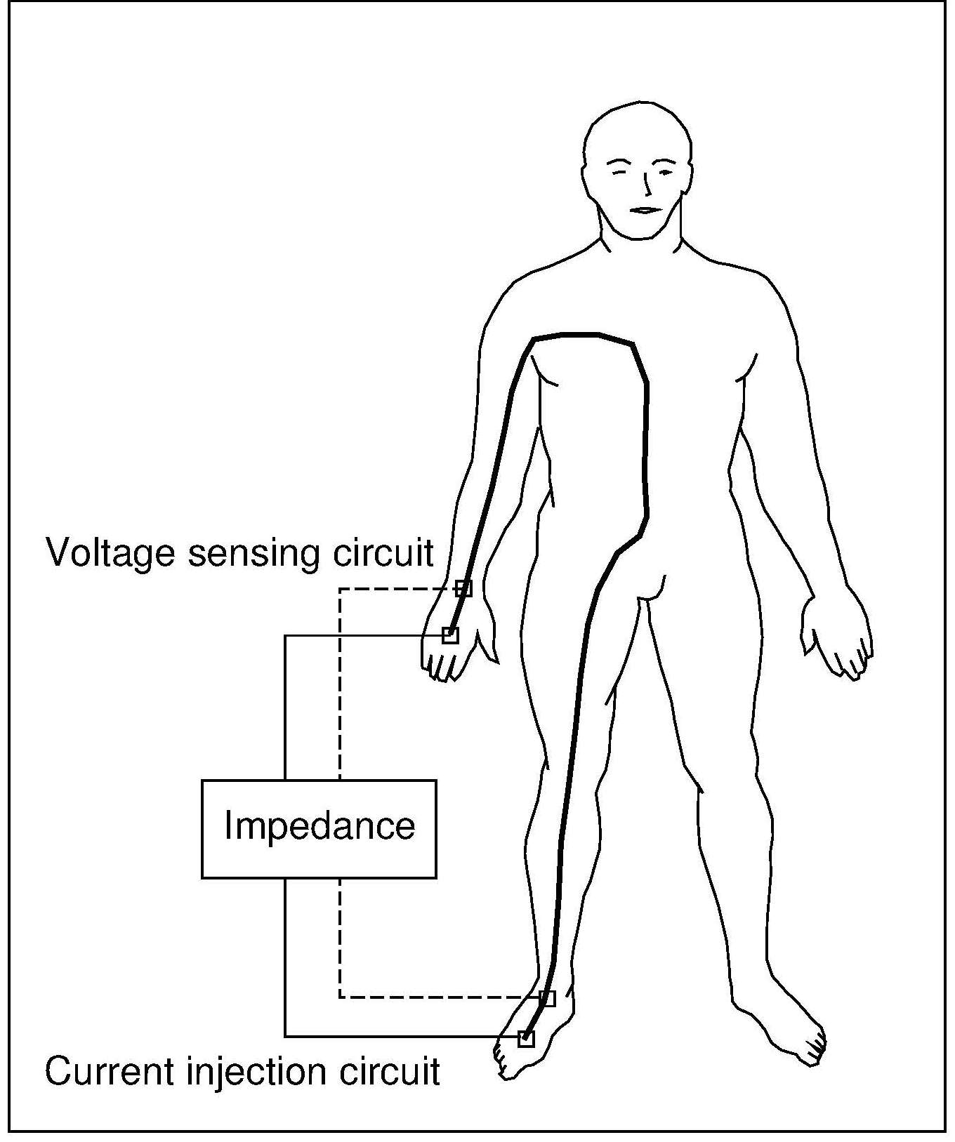

To derive fat-free mass, total body water (TBW) is predicted from raw imped­ance data by applying an appropriate regression equa­tion and the use of the assumed hydra­tion constant for fat-free mass (i.e., typically 0.732 for a healthy adult) (Section 14.3). However, as discussed earlier (see Section 14.3 and Section 14.4), many factors influence the hydra­tion of fat-free mass which have the potential to limit the accuracy of the estimates of fat-free mass from SF‑BIA data.

Theoretically, the imped­ance mea­sured at a single fre­quency (e.g., 50kHz) from a SF‑BIA device is unable to dif­fer­entiate between extra­cellular (ECW) and intra­cellular water (ICW) (or body cell mass, BCM). Many SF‑BIA devices produce pre­dic­tions of these outputs based on assump­tions that may hold true in healthy indi­viduals but not for those who are obese or sick.

14.8.2 Multiple-fre­quency bio­elec­trical imped­ance (MF‑BIA)

Multiple-fre­quency BIA devices (MF‑BIA) measure imped­ance at two or more frequencies, typically at 4 or 5 frequencies, including at least one low (most commonly 5kHz) and several higher ones (typically 50, 100, 200, and 500kHz). At lower frequencies the imped­ance to current flow allows for the deter­min­ation of the extra­cellular water space (ECW), whereas at the higher frequencies (i.e., > 50kHz) the imped­ance to current allows for the deter­min­ation of ECW and intra­cellular water space (ICW) (i.e., TBW). The volume of ICW, derived by sub­tracting ECW from TBW, can be used to estimate body cell mass (BCM) based on the assump­tion that cells are comprised of 70% water.

Several popu­lation-specific pre­dic­tion equa­tions are avail­able to predict ECW, TBW, ICW, and BCM based on refer­ence values derived from appropriate criterion methods. Never­the­less, again under­lying assump­tions may be violated in those indi­viduals with obesity and in certain clinical popu­lations, lead­ing to errors, high­lighting the importance of not accepting, without question, the output from a BIA device which uses the proprietary equa­tions of the manufacturer (Earthman, 2015).

Sex-specific BIA pre­dic­tion equa­tions, validated earlier from MF‑BIA resis­tance measures in the U.S NHANES III in 1988‑1994 (Chumlea et al., 2002), have been used to compile ratios of fat mass to fat-free mass at 5^th, 50^th, and 95^th per­cen­tiles by sex, age group, and BMI category (i.e., under­weight, normal weight, overweight, class I/II and class III obesity) for non-Hispanic persons aged 18‑90y. These fat/fat-free mass refer­ence values that account for age, sex, and BMI can be used to identify indi­viduals at risk for body compo­sition abnor­mal­ities (Xiao et al., 2018).

Measure­ments from newer MF‑BIA devices can now be made across body segments such as the limb and trunk, or across a small body region such as the muscle bed of the calf. Some MF‑BIA devices can be used in upright and supine positions so that they can be used for non-ambulatory or bed-bound persons.

14.8.3 Bioelec­trical imped­ance spec­tros­copy (BIS)

Bioelec­trical imped­ance spec­tros­copy (BIS) devices use bio­physical modeling to estimate body com­part­ments, as noted earlier; see Mulasi et al. (2015) for more details. These devices apply the electric current (typically ≤ 800µA) over a range of frequencies, from very low (e.g., 1 or 5kHz) to very high (e.g., 1000‑1200kHz), mea­sur­ing imped­ance data at ≥ 50 frequencies. This allows a more direct and indi­vidualized measure of ECW, ICW, and TBW com­part­ments com­pared with those gen­er­ated with SF‑BIA and MF‑BIA. Such measures are particularly useful in patients with altered fluid homeostasis (Mulasi et al., 2015). For those with obesity, the values for ECW and ICW can now be cor­rected using BMI as a surrogate for adiposity, thus allowing a more accurate assess­ment of body compo­sition in indi­viduals with obesity (Moissl et al., 2006).

Many validation studies of BIS conducted in healthy and clinical popu­lations are avail­able. Although good agreement at the popu­lation level can be achieved, agreement between refer­ence methods and BIS at the indi­vidual level is poor, as noted for the measure­ments from SF‑BIA and MF‑BIA devices. This limits the assess­ment of whole body masses and fluid volumes in clinical settings.

14.8.4 Bioelec­trical imped­ance vector analysis (BIVA)

Bioelec­trical imped­ance vector analysis is a graphical pro­ce­dure which uses the plot of resis­tance and reactance stan­dardized for height to create a vector that can be com­pared with gender‑ and race-specific refer­ence values from healthy popu­lation samples. BIVA can be gen­er­ated from 50kHz data. It can provide infor­mation on hydra­tion and body cell mass for patients in whom cal­cula­tion of body compo­sition is incorrect due to altered hydra­tion (Mulasi et al., 2015). In a recent study of children with severe-acute under­nutrition in Ethiopia, BIVA measure­ments successfully dif­fer­entiated between those children who were dehydrated and those with edema (Girma et al., 2021). During treatment, edematous children lost fluid whereas non-edematous children gained small amounts of fat-free tissue. Moreover, BIVA parameters correlated with bio­markers of nutritional status (Girma et al., 2018).

14.8.5 New developments in bio­elec­trical imped­ance analysis

The questionable validity of BIA approaches for the assess­ment of whole body compo­sition estimates in clinical popu­lations, especially those with abnormal body geometry or altered fluid homeostasis, has led to the use of raw BIA measure­ments per se for bedside assess­ment of nutritional status and/or clinical out­comes. Raw BIA data are inde­pen­dent of the use of regression pre­dic­tion models and assump­tions of constant chemical compo­sition of the fat-free mass, unlike the measure­ments from SF‑BIA and MF‑BIA devices. The raw BIA data used comprise single-fre­quency (50kHz) phase-sen­sit­ive measure­ments to determine: (i) phase angle, and (ii) the ratio of multifre­quency imped­ance values.

Phase angle is estimated directly by a phase-sen­sit­ive BIA device without additional conversion to specific body com­part­ments, followed by com­par­ison with popu­lation-specific refer­ence values. Phase angle is also inde­pen­dent of the body weight and height of an indi­vidual patient. The phase angle concept is based on changes in resis­tance and reactance as alternating currents pass through evaluated tissues, providing infor­mation on hydra­tion status and cell mass; for more details see Lukaski et al. (2017). Low phase angles values are typically related to more-severe illnesses and worse overall health out­comes. Currently, the major challenge of using phase angle for clinical assess­ment is the lack of consensus on the choice of cut-points to identify malnutrition (or poor clinical out­comes) (Mulasi et al., 2015).

The ratio of imped­ance mea­sured at 200kHz to imped­ance mea­sured at 5kHz — termed the imped­ance ratio or pre­dic­tion marker — is said to reflect the ratio of ECW/TBW fluid distribution, and which is currently being explored as a potential indicator of nutritional status and/or clinical out­comes. However, as stated for phase angle, the lack of a consensus on the refer­ence cut-points to use to identify malnutrition (or poor clinical out­comes) remains a major challenge for the use of the imped­ance ratio for clinical assess­ment (Mulasi et al., 2015). inves­tigations to date suggest that such refer­ence cut-points may differ depending on the popu­lation under study and the BIA device used.

Of particular inter­est is whether both phase angle (PA) and the imped­ance ratio (IR) are useful for the diagnosis of sarco­penia (with and without the presence of obesity) and malnutrition in clinical settings (Mulasi et al., 2015). Reference cut-points for both phase angle and imped­ance ratios by sex, ethnicity, and age-decade have been compiled from U.S NHANES 1999‑2004 based on BIS data. Validation with other refer­ence measures (e.g. DXA) is needed to assess whether PA/IR are appropriate for the assess­ment of nutritional status in a clinical popu­lation (Kuchnia et al., 2017).

14.8.6 Applications of bio­elec­trical imped­ance

Several popu­lation-specific regression equa­tions have been developed based on refer­ence methods capable of predicting not only fat-free mass, but fat mass and other com­part­ments from 50kHz data. Examples of these refer­ence methods include those based on a 4‑compo­nent model or dual-energy X‑ray absorp­tiometry (DXA); see Kyle et al. (2004) for more details. The regression equa­tion chosen must be matched closely to the charac­ter­istics of the subject. However, unfortunately, many devices do not specify the equa­tion programmed into their software so that the pre­dic­tion equa­tion used with the device may not be appropriate for the indi­vidual being mea­sured.

Use of a fat-free mass index has also been explored for its potential to predict nutritional status and/or clinical out­comes. The index is gen­er­ated from 50kHz data and is a height-cor­rected index of fat-free mass (i.e., fat-free mass/height squared) calculated by a stan­dardized pre­dic­tion equa­tion and com­pared with refer­ence data (Schutz et al., 2002). To date, challenges remain when applying fat-free mass index to assess nutritional status in clinical settings and more research is needed (Mulasi et al., 2015).

Interestingly, the American Society for Parenteral and Enteral Nutrition (ASPEN), does not support the use of BIA for the assess­ment of body compo­sition in the clinical setting, based on their systematic review of 23 BIA studies. Their main objections included the scarcity of data on the validity of BIA in specific clinical popu­lations, difficulties comparing studies using dif­fer­ent BIA devices, variability in the body com­part­ments estimated, and the proprietary nature of manufacture- specific BIA regression models to procure body compo­sition data. For a summary and discussion of the studies reviewed which led to this conclusion, see Sheean et al. (2020).

14.9 Computerized tomog­raphy

Computerized tomog­raphy (CT) is a high-resolution imaging technique that is widely used in clinical settings to quantify in vivo body compo­sition at the tissue-organ level. Total adipose tissue, sub­cutaneous adipose tissue, and visceral adipose tissue can be assessed. Com­puter­ized tomog­raphy can also measure skeletal muscle, indi­vidual muscle, or muscle groups, and evaluate the quality of muscle by identifying the infiltration of fat within the muscle, a condition known as myosteatosis. Computerized tomog­raphy is especially useful for inves­tigating quantitative and qualitative changes in muscle and fat in the trunk area where the use of DXA is limited.

Computerized tomog­raphy (CT) is based on the relation­ship between the attenuation of an X‑ray beam and the physical density of the tissues through which the beam has passed. The known dif­fer­ences in attenuation of X‑rays between lean soft tissue and adipose tissue can be used to distinguish these tissues as well as to determine mixtures of them. From this relation­ship, a two-dimensional high-resolution radiographic image of the under­lying anatomy of the scan area can be constructed.

The CT scanner is made up of two com­po­nents: a collimated X‑ray source and detectors, and a computer that processes the scan data and produces an X‑ray image. The subject lies on a movable platform within the scanner gantry. The designated area to be scanned is a plane through the middle of the central aperture of the gantry and parallel to the gantry. The X‑ray beam is made to rotate around the subject, gener­ating a cross-sectional “slice” through the patient. As the X‑rays pass through the tissue, the beam under­goes atten­uation, and the intensity is recorded and stored in the scanner computer. The latter then processes the stored infor­mation by using a series of complex algorithms to construct a cross-sectional image (Figure 14.11). Multiple images gen­er­ated following the movement of the patient through the scanner gantry are used to produce an integrated scan of the subject.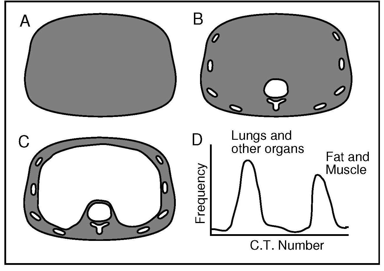

The integrated scan shows varying degrees of shading according to the magni­tude of the X‑ray beam attenuation, which, in turn, depends on the physical density of the scanned tissues. Tissues with a greater density cause a greater absorption of X‑ray energy and, consequently, a higher attenuation value. The demarcation between tissues of differing density — adipose tissue, skeletal muscle, bone, and visceral organs — can be very good.

The use of comput­erized tomog­raphy is limited by its high-dose radiation expo­sure and high cost. Efforts have been made to reduce the radiation dose by using a lower-dose protocol, essential when planning a CT scan in a child (Sorantin et al., 2013). This protocol has little deterioration in image quality (Kapur et al., 2021). Single-slice scanning can also be used to reduce the radiation dose.

A new technique with extremely low radiation expo­sure, shorter scan time, and relatively low cost com­pared to whole body CT, termed “peripheral quantitative computer tomog­raphy” (pQCT) has been developed. This new technique has been used primarily to inves­tigate bone mineral content and to assess bone fragility in older patients (Jiang et al., 2018). However, despite these efforts, radiation expo­sure is still high, restricting the use of CT images for clinical use during disease treatment rather than for body compo­sition assess­ment.

14.9.1 Application of comput­erized tomog­raphy

The method has several uses. It can be used to assess changes in the visceral organ mass in under­nutrition and obesity, to portray the distribution of sub­cutaneous versus visceral adipose tissue, and to establish bone density in osteopenia (Heymsfield et al., 1987). New techniques with improved spatial resolution can be used to detect and measure fat in areas of the body where fat is not physiologically stored, such as the liver, pancreas, heart, and skeletal muscle. The fat deposited in these areas is termed visceral ectopic fat and is known to contribute to the development of coronary artery disease as well as other cardio­vascular disorders (Neeland et al., 2019).

The region of special interest for the study of body compo­sition using CT scans is the third lumbar vertebra (L3). This is the region where a single image of a cross- sectional area provides the best correlation of whole-body skeletal muscle volume. The validity and accuracy of body compo­sition measure­ments by CT based on cross-sectional area of tissues have been validated by studies of human cadavers, although no validation of the cal­cula­tion of tissue volume has been performed (Fosbøl & Zerahn, 2015).

Increasingly, CT scans are also being used to identify CT-defined sarco­penia, a condition associ­ated with a decrease in muscle mass and function which, although originally described in the elderly, is also of concern among the chronically ill nonelderly (Peterson & Braunschweig, 2016). To date, how­ever, there are no clear diagnostic cutoff values for CT to identify sarco­penia based on skeletal muscle mass, which has limited the applic­ation of CT for clinical use.

14.10 Magnetic resonance imaging

Unlike computer tomog­raphy or DXA, magnetic resonance imaging (MRI) does not use ionizing radiation so that the technique can be used on infants, and for long-term follow-up when multiple scans on the same person are required. The MRI technique is mainly used to evaluate the quantity and distribution of adipose tissues and skeletal muscle mass, although it can also detect changes in body compo­sition, even in the presence of small body weight changes (Lemos & Gallagher, 2017). In older equipment, scanning times of 10min were necessary, but in more modern equipment, this has been reduced to under 2min. Never­the­less, the MRI technique requires tech­nical expertise, is expensive, and the equipment is bulky (Prada & Heymsfield, 2014).

Magnetic resonance imaging uses dif­fer­ences in the nuclear magnetic resonance properties of hydrogen atoms in organic and non-organic environments to distinguish signals origin­ating from fat, fat-free mass, and free water. The hydrogen protons behave slightly dif­fer­ently in adipose versus lean tissues. The dif­fer­ences are in the relaxation time that it takes for the nuclei to release the radio-fre­quency-induced energy and return to a random con­figur­ation. These dif­fer­ences can be used to map the distribution of adipose versus lean tissue in the body (Ross, 1996).

The imaging process involves placing the subject in a very strong magnetic field. Some of the nuclei in the body attempt to align themselves relative to the applied field. The effect is particularly marked for ¹H protons. Only a small fraction of the protons become aligned, but they are suffi­ciently numerous for the effect to be detectable when the field is removed or altered. It is then that the dif­fer­ences between the lean and adipose tissue become apparent.

14.10.1 Application of magnetic resonance imaging

Magnetic resonance imaging is often used in clinical settings, when, instead of using whole body imaging which is time consuming and expensive, sectional body compo­sition studies that often employ the L3 lumbar vertebra as the landmark, are used. This landmark has the highest correlation with whole body skeletal muscle and visceral fat volume. Alternatively, to identify sarco­penia in older adults, a single-slice at the mid-thigh level can be used as this provides a good estimate of skeletal muscle and fat volume in the thighs, and correlates with clinical criteria; see Lee et al. (2019) for more details.

14.11 Dual energy X‑ray absorp­tiometry

Dual-energy X‑ray absorp­tiometry (DXA) is a technique that can be used with indi­viduals (except pregnant women) across the entire age range and at relatively low cost. DXA is widely used to assess body compo­sition, with an overall precision that exceeds that of any other body compo­sition method (Prada & Heymsfield, 2014).

With the latest generation of densitometers, body compo­sition can be assessed with a single whole-body scan so that radiation expo­sure is low with a minimal acquisition time. In addition, the newer instruments enable indi­viduals with extreme obesity to be scanned.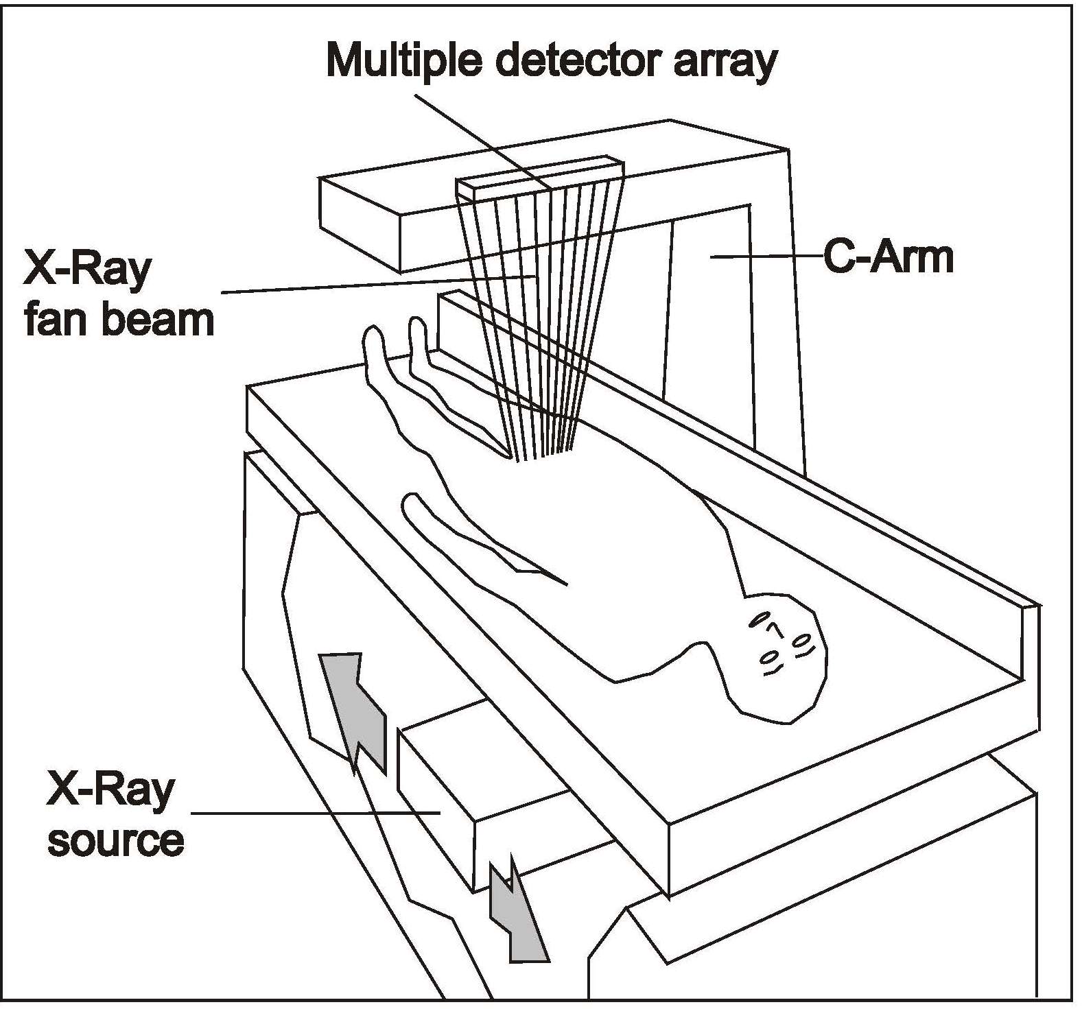

Modern DXA scanners use an X‑ray source, a detector, and an inter­face with a computer system for imaging the scanned area of inter­est. The source gen­er­ates X‑rays at two dif­fer­ent energy levels — 40KeV and 70‑100KeV. These pass through the body and are identified by the photon detector that measures the amount of photon energy absorbed at the two energy levels by the soft tissue and bone. Low-density material (i.e., soft tissue) allows more photons to pass through, so they attenuate the X‑ray beam less than materials with a higher density, such as bone. An image is gen­er­ated as the photon detector measures the dif­fer­ential attenuation (or absorption) of the low and high X‑rays by the soft tissue and bone. Only in regions of the body where no bone is present can measure­ments of the relative pro­por­tions of fat and lean tissues be made; see Prada & Heymsfield (2014) for more details.

During an inves­tiga­tion, the subject, on a movable bed, is scanned recti­linearly from head to toe. The X‑ray source is situated beneath the scanning bed, and scans usually take from 5‑20min depending on type of scan and software selected (Figure 14.12).

The accuracy of DXA results is influenced by both tech­nical and bio­logical factors; these are sum­ma­rized in Figure 14.13. The tech­nical factors include dif­fer­ences in machine cali­bra­tion pro­ce­dures, the protocols used in demarcating the regions (arms, legs and trunk) in estimates of body compo­sition, the positioning of the subject on the scanning bed, and the effect of clothing. Sources of biological variability that can affect accuracy include hydra­tion status because the hydra­tion of fat-free mass is assumed to be constant (i.e., about 73%). Hence, when changes in hydra­tion status are large (i.e., higher than 5%), as may occur in the presence of diseases with water retention (e.g., heart, kidney or liver failure), the fat-free mass is over-estimated (Nana et al., 2015). In older DXA models, obesity was also a factor limiting accuracy, but newer instruments allow larger and heavier indi­viduals to be scanned. Finally, the ability to compare body compo­sition estimates between DXA manufacturers is limited because of variations in the hardware and software packages used by manufacturers, high­lighting the urgent need for universal cali­bra­tion of DXA machines (Prada & Heymsfield, 2014).

Several inves­tigators have tried to establish the absolute accuracy of gross measure­ments of body compo­sition in vivo performed using DXA. Many of these studies have examined correlations between measure­ments made by DXA on pig cadavers and sub­sequent direct chemical analysis; results have been mixed (Jebb, 1997).

14.11.1 Applications of DXA

Dual-energy X‑ray absorptiometryis now the primary method for gener­ating accurate data on bone mineral content and density for the diagnosis of osteo­porosis (see Chapter 23 for more details). DXA is also widely used to assess body compo­sition, with an overall precision that exceeds that of any other body compo­sition method (Prada & Heymsfield, 2014). Both total and regional estimates of the three body com­part­ments — fat-free mass, body fat, and bone mineral content — can be deter­mined. However, DXA does not have the ability to discriminate between visceral, sub­cutaneous, and ectopic fat present in organs such as liver or muscle.

Estimates of the appendicular skeletal muscle mass (ASM) can be obtained from DXA. These estimates are gen­er­ated by summing the amount of lean soft tissue (LST) of the arms and legs, as they are composed mainly of muscle (except for a small amount of connective tissue and skin) (Prada & Heymsfield, 2014). From these estimates, the ASM index can be calculated by dividing the arm and leg lean soft tissue (LST) by height squared. Both the ASM and the ASM index values are considered the gold stan­dard method for the diag­nosis of sarco­penia. For pub­lished cutoff points to define sarco­penia based on DXA, see Earthman (2015).

In a systematic review based on eight DXA studies by the American Society for Parenteral and Enteral Nutrition (ASPEN), DXA was recom­mended for the assess­ment of fat mass in patients with a variety of disease states, but not for fat-free mass (Sheean et al., 2020). They stressed that the validity of DXA for assess­ment of fat-free mass in any clinical popu­lations remains unknown. Clearly, addi­tional research is needed to evaluate the validity of DXA for quantifying fat-free mass in clinical populations.

14.12 Ultrasound

Diagnostic ultra­sound, also called sonography, is an imaging technique used in clinical settings to measure various tissue thicknesses, including muscle, bone, and sub­cutaneous and visceral adipose tissue. The device is portable, low cost, and capable of making fast and noninvasive regional estimates of body compo­sition with no expo­sure to ionizing radiation. Conse­quently, this scanning technique can be used in children and pregnant women and is suitable for large epidemiological studies, although the results gen­er­ated are highly dependent on the skill of the operator.

The ultra­sound technique involves the use of high-fre­quency sound waves from a transducer. These penetrate the skin surface and pass through the adipose tissue until they reach the muscle tissue. At the adipose-muscle tissue inter­face, a pro­por­tion of the sound waves are reflected back to the transducer as echoes. Hence, the transducer both transmits and receives the ultra­sound. The degree of reflection is dependent on the changes in acoustic imped­ance (i.e., the product of tissue density and acoustic velocity) between two tissue inter­faces. The higher the acoustic imped­ance, the stronger the gen­er­ated reflection, and thus, the better the quality of the image.

The acoustic imped­ance of fat and muscle are somewhat similar and much lower than bone which has a relatively high acoustic imped­ance; air has almost no imped­ance. Conse­quently, there is a weaker echo at the fat-muscle inter­face than at the muscle-bone inter­face. When the transducer receives the beam, it converts the echo into electric signals to form a two-dimensional image. The relative strength, or amplitude, of echoes is apparent from the brightness of the image on the computer screen, with strong reflect­ions appearing white, weaker reflections grey, and no echoes black. As a result, a grey-scale image is produced with white borders for the skin-subcutaneous fat and muscle-bone inter­faces and a visible, but less distinct border for the fat-muscle inter­face; see Wagner (2013) for more details.

However, the inter­pretation of ultra­sound images is difficult and depends on the tech­nical expertise of the operator who must identify the inter­faces and measure the thickness of the tissue layer of interest using electronic calipers. Care is needed to identify and place the two caliper points at the boundaries of the tissue to be mea­sured. An automated discrimination method is avail­able to identify the tissue boundaries for some ultra­sound devices, although studies comparing the automated method with the manual discrimination are limited (Wagner, 2013).

To use ultra­sound, the measure­ment site is marked with a water-soluble transmission gel that provides acoustic contact without depression of the dermal surface. The high-resolution transducer is then placed without loss of contact with the skin so that the ultrasonic beam is perpendicular to the tissue inter­faces at the marked site. A transducer receives the echoes and translates them into depth readings viewed on a computer screen. Thicknesses of 100mm or more can be mea­sured, and density inter­faces can be detected with an accuracy of 1mm. The tissue is not com­pressed, thereby eliminating errors associ­ated with variations in the com­press­ibility of skinfolds (Fanelli & Kuczmarski, 1984).

14.12.1 Applications of Ultrasound

Visualization of a fetus during a prenatal examination is the most familiar applic­ation of ultra­sound. However, ultra­sound is also used to measure the quality and quantity of skeletal muscle mass, an index of lean soft tissue, in the elderly, patients with cystic fibrosis, and patients confined to bed rest (Prada & Heymsfield, 2014). Alternatively, measure­ment of the thickness of sub­cutaneous fat can be used to monitor changes in body compo­sition of hospital patients receiving nutritional support.

In general, the ultra­sound method provides a reasonable estimate of adipose tissue thickness in humans, com­pared to total body elec­trical conduc­tivity (TOBEC) and skinfold caliper techniques (Fanelli & Kuczmarski, 1984). For obese persons especially, ultra­sound may be superior to skinfold caliper techniques for mea­sur­ing sub­cutaneous fat (Kuczmarski et al., 1987). The method can also be used to measure thickness of other tissues such as muscle and bone, as noted earlier; for more details see Mayans et al. (2012) and Karjalainen et al. (2008).

An ultra­sound system has also been designed specifically for body compo­sition which could be the user-friendly ultra­sound alternative to skinfolds and other field methods for esti­mat­;ing per­cent­age body fat (Wagner, 2013). However, currently the diverse technology across the commercially avail­able devices and the lack of stan­dardized measure­ment protocols makes it difficult to compare results across studies (Lee et al., 2019). The American Society for Parenteral and Enteral Nutrition (ASPEN) did not recommend the use of ultra­sound to assess body compo­sition in a clinical setting, based on their systematic review of seven studies (Sheean et al., 2021). More research is needed to develop consensus on the optimal method to conduct ultra­sound measure­ments and to gen­er­ate popu­lation-specific refer­ence data so that the method can be used to assess lean tissue and diagnose malnutrition in a clinical setting (Earthman, 2015).

14.13 Summary - Method com­par­isons

Increasingly, clinicians are using the more robust and reproducible in vivo methods de­scribed in this chapter to measure body compo­sition in view of the limit­ations of BMI as a proxy for adipos­ity and the recog­nition that dif­ferences in body compo­sition are associ­ated with an increased risk of diseases across the life­span. Such diseases may include AIDS-associ­ated wasting, dia­betes, osteo­porosis, sarco­penia, cardio­vascular disease, and anorexia nervosa. Even during early infancy, changes in body compo­sition (both fat and fat-free mass) can provide more under­standing of the init­iators and mediators of the develop­mental origins of adult cardio­metabolic disease (McMillen et al., 2005).

However, no single in vivo method has the ability to track body compo­sition accurately from infancy to adulthood; all have strengths and technological limit­ations. Fields and co-workers (2015) have com­pared selected in vivo methods for assessing whole-body compos­ition across the life span; details are shown in Table 14.6.

Table 14.6. Comparison of selected methods for determining whole-body compo­sition across the life span.
C, cost limits widespread use; D, difficult to perform but still possible; I, impractical (maybe impossible) due to age- and compliance-related issues; NA, not applicable; NV, not valid or little data exist in determining validity; P, probative data support its validity, precision, and reliability in this popu­lation; PL, possible—limit­ations exist in inter­pretation to whole-body compo­sition; R, radiation involved, marginally small although institutional review boards may limit its use; UE, may be unethical due to radiation; VA, validity is ambiguous or weak in this popu­lation. ^agap exists between 6mos and 2y.

Method	Infancy (< 6mo)	Childhood (2‑6y)	Adolescence (7‑17y)	Adulthood (≥ 18y)
Hydrostatic weighing	NA	I	D|I	P
Air displace­ment pleth­ysmog­raphy	P	Pa|D	P	P
Whole-body counting for K	UE|C	UE|C	UE|C	D|C
Dual-energy X‑ray absorp­tiometry	D|R	D|R	R	P|R
Bioelec­trical imped­ance	VA|NV	VA|NV	VA	P
Computed tomog­raphy	UE	UE	UE	UE
Isotope dilution	I	D|P	D|P	P
Magnetic resonance	D|C	D|I|C	D|I|C	P|C
Ultrasound	NV	NV	NV	NV

When compiling this table, the invest­igators con­sid­ered the techno­logical limit­ations of each method, and the follow­ing four criteria:

• Cost of the measure­ment / device
• Level of patient cooper­ation needed for accurate results
• Feasi­bility in obtain­ing an interp­retable result given the patient’s age
• Apprec­iation of the age of the patient relative to the assump­tion of the under­lying prin­ci­ples in the chosen method.

Based on their review of the methods listed for whole-body assess­ment in Table 14.6, Fields et al. (2015) chose air dis­place­ment pleth­ys­mography (Section 14.6.3) as the method with the highest degree of accuracy and reli­abil­ity and with the least degree of tech­nical error across the life span. Cur­rently a “suite” of air dis­place­ment pleth­ysmo­graphic devices are avail­able which can be used to track and monitor body compos­ition from birth, into adol­escence and through­out adult­hood; they are described in Section 14.6.3 and have also been reviewed by Fields et al. (2015).

Acknowledgments

RSG is grateful to Michael Jory for the HTML design and his tireless work in directing the trans­ition to this HTML version.