Book

Kirkpatrick S.     Validity in
Dietary Assessment

3rd Edition    August, 2025


Abstract

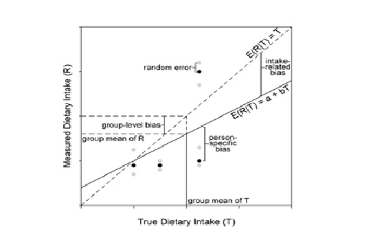
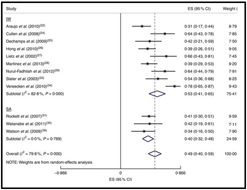
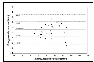
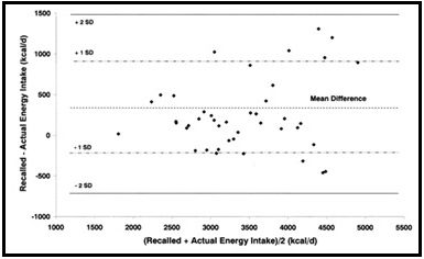
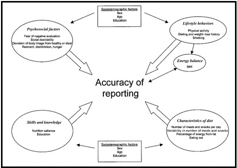
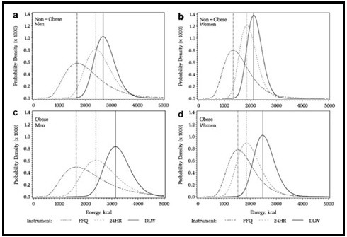
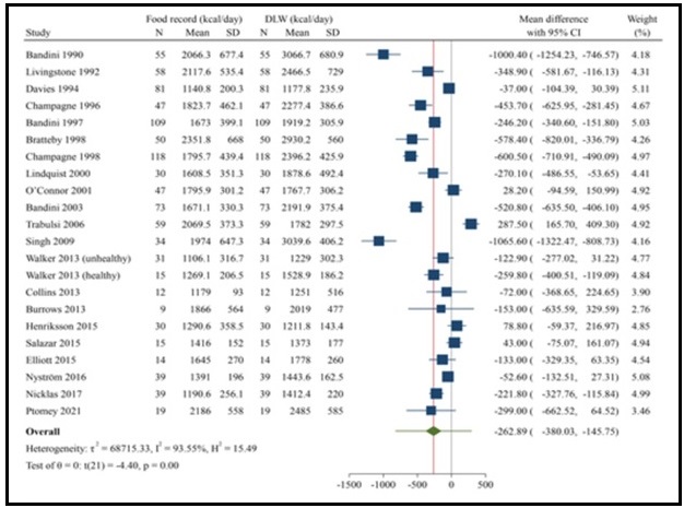
Validation describes the process to determine whether a method provides useful information for a given purpose and context. In developing or adapting a dietary assessment method, face and content validity may be assessed with members of the target popu­lation and experts in the field to inform and refine the method. Once a method has been developed, it is critical to consider the extent to which it has construct and criterion validity for a given purpose and popu­lation. Construct validity indicates whether the method measures what it is intended to measure, whereas criterion validity refers to the method's accuracy in doing so. Criterion validity is best assessed by comparison of the method under evaluation to an unbiased measure. However, because of the logistical and financial challenges in implementing unbiased measures of dietary intake, especially in large studies, the method being evaluated may be compared to another error-prone measure, usually a self-report method such as weighed food records or multiple 24h recalls.

The concept of validity operates on a continuum. Consequently, a given study does not serve to indicate that a method is valid or invalid but rather, provides evidence that a dietary assessment method has a sufficient level of validity for a given purpose. Inferences about the degree of validity should be specific to the popu­lation(s) and context(s) studied; for example, a method found to have a certain level of validity for use with adults may not have the same level of validity when used with adolescents. Furthermore, the full body of evidence available about a method, including evidence on different types of validity and using different study designs, should be considered when making decisions about whether a method has adequate validity for a given purpose and in interpreting the data collected. Under­standing the extent of the validity of various methods also helps identify strategies to improve dietary assessment.

This chapter discusses the evaluation of the validity of dietary assessment methods, with a focus on the evaluation of criterion validity using error-prone and unbiased reference measures. CITE AS:     Kirkpatrick S,     Validity in Dietary Assessment https://nutritionalassessment.org/Validity/
Email: skirkpat@uwaterloo.ca
Licensed under CC-BY-4.0
( PDF )

7.1 Assessing validity in dietary assessment

In developing or adapting a dietary assessment method, face and content validity may be assessed with members of the target popu­lation and experts in the field. Face and content validity assess whether the method is well constructed and grounded in an under­standing of the phenomenon we are intending to measure (Frongillo et al., 2019; Kirkpatrick et al., 2019). To ensure face and content validity, a Delphi technique (Dalkey and Helmer, 1963; Hsu and Sandford, 2007) may be used to develop consensus among experts on foods and beverages for inclusion in a questionnaire to maximize content validity. The face and content validity of methods may also be assessed with members of the target popu­lation, for example, using cognitive inter­views. Subar et al. 2007 used observation by a cognitive inter­viewer to glean insights into how to structure the initial pass of a multi‑pass online self-administered 24h recall system.

However, face and content validity do not indicate whether the method measures the construct of interest and how accurately it does so, necessitating assessments of construct and criterion validity. Construct validity indicates whether the method measures what it is intended to measure. One way to assess construct validity, for example, is to examine whether a method can differentiate between groups of people, such as men and women, who are known to have differences in dietary intake (Guenther et al., 2008).

Criterion validity is assessed by comparing data from the method being evaluated to a reference method. Examining the criterion validity, or accuracy, of dietary assessment methods is the focus of much validation research within nutrition because under­standing the extent to which the data collected are affected by error (Chapter 5) is essential for matching methods to research questions, as well as the robust interpretation of results. Strictly speaking, assessing criterion validity of a dietary assessment method requires an evaluation of the accuracy with which it captures true intake. However, it is difficult to obtain unbiased dietary intake data to serve as the criteria for comparison. This is particularly true when interest is in usual or habitual dietary intake, which is often the focus of dietary assessment (Chapter 3). For example, in surveillance, interest is in whether intake is aligned with dietary guidance on average over time, not on a given day, and in epidemiology, the focus is typically on associations between usual intake of given dietary components or dietary quality and a disease outcome. Similarly, in intervention studies, the goal is usually to shift dietary intake for the long‑term rather than only a short period.

Measuring true usual intake is very challenging. Nonetheless, studies drawing upon obser­vational designs or feeding protocols may collect data that are closely reflective of true intake. For example, evaluations of 24h recall and food record protocols and platforms have sought to measure true intake by surreptitious observation or weighing of foods and beverages taken by or served to participants along with plate waste. A feeding study design has also been used to evaluate the use of video capture to identify foods consumed (Lozano et al., 2023). However, such studies are typically feasible for only short periods of time, so these designs are generally amenable to evaluating the validity of short‑term methods like 24h recalls and food records for capturing true intake on a day or over a few days. They are not typically used to assess the criterion validity of methods that aim to capture habitual intake over a longer period, such as a month or a year. Furthermore, even if actual food intake, monitored using unobtrusive observations and weighing, compares favorably with data from a self‑report method such as 24h recalls administered to the same individuals during a consistent period, these findings may not generalize to studies that aim to capture usual intake over a longer period outside of controlled settings. Additionally, due to the costs and practical considerations, evaluations of criterion validity using observation and feeding protocols generally involve a limited number of individuals, with potential implications for representativeness and generalizability.

Discovery of bio­markers that can be used to measure exposure to dietary components is an ongoing and active area of research (Brouwer‑Brolsma et al., 2017; Chakraborty et al., 2025; Maruvada et al., 2020). Though expensive and burdensome, recovery bio­markers (Kaaks et al., 2002) (Chapter 15, Box 15.4) are particularly useful for assessing the criterion validity of dietary assessment methods. Recovery bio­markers are biological products in body fluids or tissues that are directly related to intake and are not subject to substantial differences in how they are metabolized across individuals. Recovery bio­markers measure total excretion of a marker over a defined period and therefore, provide an indication of absolute intake (Jenab et al., 2009; Kaaks et al., 2002). Recovery bio­markers have been identified for energy intake over a 10‑to‑14‑day period if individuals are in body weight balance, based on doubly labeled water (Schoeller and Hnilicka, 1996), and for protein (Bingham, 2003), potassium (Tasevska et al., 2006), and sodium (Day et al., 2001; Luft et al., 1982, Mickelsen et al., 1977) based on 24h urine collection. Recovery bio­markers provide nearly unbiased estimates of intake and can therefore be thought of as criterion measures, though some systematic error is possible, for example, due to incomplete specimen collection and/or lab errors. Recovery bio­markers are affected by within‑person random error that, as described for short‑term dietary assessment data such as that from 24h recalls, can be addressed using repeat measures and statistical modeling.

Recovery bio­markers have been used in several validation studies to evaluate intake data from 24h recalls, food records, and food fre­quency question­naires; details are given in Section 7.5. Such studies have improved our under­standing of the extent to which different types of measure­ment error affect data from various dietary assessment methods, that is, the structure of the measure­ment error (Kipnis et al., 2003). Results of these bio­marker studies have emphasized that energy under­estimation occurs in all dietary assessment methods, leading to the recommendation not to rely on self‑reported dietary data to estimate energy intake (Subar et al., 2015). Findings from such studies also indicated recalls capture absolute intake of the dietary components investigated with less bias than fre­quency question­naires (Freedman et al., 2014, 2015; Kipnis et al., 2003; Subar et al., 2003), and were part of the impetus for the development of self-administered 24h recall systems described in Chapter 3. Such self-administered systems enhance the feasibility of collecting repeat recalls in very large studies, such as cohorts, with the aim of improving the capacity to identify diet and disease associations by recording more accurate dietary intake data. Bio­marker-based validation studies have also informed new analytic approaches by combining data from different self‑report methods to improve the estimation of diet‑disease associations (Carroll et al., 2012; Freedman et al., 2018).

Additional categories of bio­markers, such as predictive and concentration bio­markers, may respond to intake of a dietary component. Predictive bio­markers are like recovery bio­markers in that they show a dose‑response relationship with intake, but their overall recovery is lower (Tasevska et al., 2005). Concentration bio­markers do not reflect absolute levels of intake but are correlated with intake (Jenab et al., 2009). Such bio­markers are increasingly used in validation research, with substantial ongoing effort to discover new bio­markers of intake for nutrients, foods, food groups, dietary patterns, and other components such as alcohol and caffeine (Brouwer‑Brolsma et al., 2017; Chakraborty et al., 2025; Maruvada et al., 2020).

The relative validity of dietary assessment methods may be assessed using biased or error‑prone reference methods. Such methods may be thought of as comparison rather than criterion measures to differentiate them from unbiased reference methods such as observation or recovery bio­markers. In this approach, the "test" dietary method is evaluated against another "reference" dietary method administered to the same individuals. For example, a fre­quency questionnaire may be assessed by comparison with weighed food records, spaced out over a period analogous to that captured by the questionnaire. The comparator is generally a dietary method, chosen, ideally such that errors between the two dietary methods being compared are independent, though this is often not the case, especially when two self‑report methods are compared.

In addition to validity, equivalence is an important consideration in terms of whether a given method performs similarly in different popu­lations. For example, an online interface to complete 24h recalls should be assessed to ensure it performs similarly in the different popu­lations in which it is intended to be used. This is particularly critical for multicenter trials, in which cultural or language differences may influence the way in which individuals respond to a dietary assessment method. Relatedly, there is a need to broaden the diversity of samples used in studies that use true criterion measures, such as recovery bio­markers. Participants in validation studies have often been drawn from convenience samples or consist of highly motivated volunteers who may provide more accurate responses and/or have different dietary practices than the study popu­lation, with important implications for generalizability. Careful interpretation and reporting of validation studies is thus critical. Statements regarding the validity of a method should reference the popu­lation and context in which it was evaluated (Frongillo et al., 2019; Kirkpatrick et al., 2019) .

Furthermore, statements regarding the validity of a method should be specific with respect to the dietary components that have been investigated. Finding that a method performs well for some subset of dietary components does not imply that it performs well for all dietary components. The opposite is also true. Errors in the estimation of energy intake compound across foods and beverages consumed (Subar et al., 2015), which is a major concern because total energy intake is poorly estimated by self‑report methods. Poor estimation of energy intake by a method, however, does not necessarily equate to poor estimation of intake of all dietary components, nor of dietary composition. Studies using recovery bio­markers, as well as an obser­vational design, indicate that bias in reporting is differential across dietary components (Freedman et al., 2014; 2015; Garden et al., 2018).

Biases in estimated intake can arise from the omission of foods truly consumed, reporting of foods habitually consumed but not consumed during the reporting period, reporting of foods not habitually consumed because of social desirability bias, and errors in portion size estimation. These errors may be additive or may cancel each other out to some extent, depending on the nutrients and foods of interest. For example, in an obser­vational feeding study with 302 women with low income, overestimation of portion sizes appeared to counteract the effects of omitted foods on estimated intake to some extent (Kirkpatrick et al., 2022). Depending on the study design, it may be possible to consider various contributors to bias and how they interact to impact the accuracy of estimated intakes. However, Whitton et al., 2022 have noted that the lack of consistency in how error is reported in different studies has hampered our under­standing of how the overall accuracy in estimated intakes is affected by interactions among the contributors to error. As discussed in Chapter 5, the lack of accuracy of portion size estimation continues to be an important source of error in self‑report dietary intake data (Whitton et al., 2022) and efforts to improve this facet of dietary assessment are ongoing. A 2020 review identified the need for high quality validation studies in this area (Amoutzopoulos et al., 2020).

Manuscripts reporting on validation studies often conclude that a method is "valid" (Lombard et al., 2015) which suggests a dichotomy in terms of methods being valid or not. This is not appropriate in the case of self‑report dietary assessment methods that universally capture intake with error. While authors may use cutoffs to determine whether observed statistics meet thresholds for high or moderate validity, for example, these thresholds are arbitrary, and the full results should be examined to make decisions about which methods to use and how to interpret the data they produce. Drawing upon the "Strengthening the Reporting of Obser­vational Studies in Epidemiology-nutritional epidemiology" (STROBE-nut) statement (Lachat et al., 2016). Kirkpatrick et al., 2019 provide a checklist intended to encourage complete and transparent reporting of validation studies. A holistic consideration of validity also considers reproducibility and other elements of reliability (Chapter 6).

7.2 Design of relative validity studies using error‑prone reference measures

This discussion begins with studies using error‑prone reference methods to assess relative validity, prior to discussing considerations associated with the use of unbiased reference measures including obser­vational feeding studies and recovery bio­markers as criterion markers. Several factors summarized below must be considered in the design of validation studies. For detailed discussions, see Frongillo et al., 2019 and Kirkpatrick et al., 2019 .

7.2.1 Study objective and time frame

The reference dietary method chosen must measure similar parameters over the same time frame as the test method. Four possible levels of objectives for dietary assessment protocols have been defined, as discussed in detail in Section 3.3.

Assessment of the relative validity of a method designed to determine usual food or nutrient intakes of individuals over the distant past is especially difficult. As an alternative, validation studies of current intake have sometimes been conducted as a proxy for past diet, on the assumption that it is related to past intake. However, this may not be the case. Studies have reported a tendency for the recall of past diet to be affected by recent consumption, termed a "recency" effect (Byers et al., 1983; Rohan and Potter, 1984). However, Ambrosini et al., 2003 compared intakes based on four 7d food records completed by participants in a cancer prevention trial at baseline, to a food fre­quency questionnaire completed 10y later. The fre­quency question­naire was modified to ask about usual intake at baseline, with the authors finding that mean intakes of most nutrients did not differ between the two methods.

Nonetheless, the health status of the individuals of interest is an important consideration, especially in case‑control studies. Attempts should be made to evaluate the dietary method with representatives of both the cases and the healthy controls. Retro­spective reports of diets obtained from individuals with serious illnesses may be biased by recent dietary changes (Friedenreich et al., 1992). For instance, Jain et al., 1980, in a prospective study of diet and cancer, showed that newly diagnosed cancer patients who were asked to recall their food intake 6mo ago under­estimated the earlier intakes that had also been recorded 6mo previously. Among the controls, however, there was little difference between reported and recalled intakes. The authors concluded that the recalled intakes of the cancer patients in this study were influenced by the current intakes, distorting the recall. In their study of contemporaneous and retro­spective estimates of food intake using a dietary history, Van Staveren et al., 1986 also concluded that current food intake affected reporting of past food intake.

7.2.2 Sequence and spacing of test and reference methods

The test and comparator methods should capture the same construct over the same period. For example, to evaluate a fre­quency question­naire intended to capture usual intake over a month relative to 24h recalls, decisions regarding the number and timing of recalls should be tailored towards reflecting usual intake over that same period. Depending on study resources, multiple recalls that capture weekdays and weekend days and that are spaced over the month may be administered.

It is also important to consider whether completion of one method may influence responses to the other. For example, when using weighed food records as a reference, the process of weighing and recording foods may enhance accuracy in reporting intake using other tools, such as fre­quency question­naires. Consistently, Willett et al., 1985 showed that food fre­quency question­naire results correlated better with data from four 1wk weighed records completed over the course of a year, if the food fre­quency question­naire was administered after, rather than before, the reference method. Recording intake in real time may also lead to reactivity, such that eating practices are changed, with possible biases in the data from the test and comparison methods.

Too long a time interval between the test and reference methods may introduce seasonal effects on food intake. Such an effect may be especially evident in contexts in which food availability is particularly affected by seasonal shifts, such as in low‑income countries (Section 6.2).

7.2.3 Independent errors

Errors in the reference dietary method should be independent of those in the test method and of the true intake (Kipnis et al., 2001; 2002). As a result, the selected reference dietary method should be different from the test method. For example, the two methods should not both rely on memory or use the same method for estimating portion sizes.

Even when precautions are taken, the reference dietary method is rarely free from all sources of error (Kaaks and Riboli, 1997; Kipnis et al., 2001; 2002). Systematic error is made up of both intake‑related and person‑specific biases. An intake related bias usually reveals itself in a "flattened" slope of the regression of reported intake on true intake. As an example of an intake‑related bias, persons with low consumption of foods who are encouraged to eat more for health reasons, may over‑report their true intake. In contrast, those with high intake of foods who are recommended to restrict their food intake, may tend to under­report their intake. Person‑specific bias may be caused by individual character­istics. It is possible that some individuals may under or overreport in their responses to both the test and reference methods, leading to artificially high correlation coefficients between the two different methods. Figure 7.1 provides an overview of the Kipnis measure­ment error model (Kipnis et al., 2003) that provides a framework for conceptualizing different sources of error (Kirkpatrick et al., 2022).
Figure 7.1
Figure 7.1. The Kipnis measurement error model describes the relationship between true usual dietary intake (T) and an error-prone measure (R). It assumes the measure is correlated with truth, but not perfectly. The figure illustrates the main features of the Kipnis model. The black circles represent the long-run average (in statistical language, the expectation) of repeated applications of the measure to particular individuals in the group (only a few individuals are represented in the figure), whereas the grey circles represent particular applications of the measure. Mismatches between particular measurements and their long-term average are considered random errors.

The dashed 45-degree line labeled “E(R|T) = T” is the line of identity. The solid line, labeled “E(R|T) = a + bT”, is the linear regression line plotted through the black circles (seen and unseen) for the entire group, reflecting that correlation between R and T describes the strength of their linear relationship. The regression equation provides a predicted value of the measure R in terms of the true intake T. However, not all the black circles will fall on the regression line, because the Kipnis model assumes usual intakes and long-run averages of the measure are not perfectly correlated. The differences between the regression equation and a given person’s black circle is defined as their “person-specific bias” and reflects that two individuals with the same usual intake might systematically report their intake differently.

The vertical difference between the line of identity and the solid regression line at a particular value of T is the “intake-related bias” — the average difference between the measured values and T, the true usual intake for those persons. The intake-related bias depends upon the magnitude of usual intake. This feature mirrors the “flattened slope” phenomenon such that persons with low usual intake tend to have measured intakes that exceed their true intakes (seen in the lower left corner of the figure), and persons with high usual intake tend to have measured intakes that fall below their true intakes (seen in the upper right corner). Of interest is the intake-related bias at the group mean of T — the vertical dashed line in the Figure. The vertical line intersects the solid line at the group mean of R, and intersects the dashed line of identity at the group mean of T. Thus, the vertical difference between the two is the group-level bias. If the regression line and the line of identity intersect at the group mean of T, then there is no group-level bias, though other systematic and random errors may be present.
From Kirkpatrick et al., 2022).

Novel methods such as web‑based recalls or pre‑coded diaries are often purposely compared to methods with similar character­istics, such as inter­viewer-administered recalls and weighed records, respectively. Such comparisons can lend insight into the impact of changes in mode of admin­istration and/or question­naire structure, for example, to assess whether a reduction in respondent burden is worth a given reduction in accuracy. Ideally, to assess validity, the test method is also evaluated in an obser­vational feeding study (Section 7.4). or relative to recovery bio­markers (Section 7.5), though due to the cost and logistical considerations in conducting such studies, the samples are often small and as mentioned, there may be important considerations related to generalizability, for example, based on findings with highly motivated volunteers or convenience samples.

7.2.4 Sex and age

Sex and age have been shown to be associated with error in reported intakes in bio­marker‑based studies (Burrows et al., 2020; Freedman et al., 2014; 2015). Further, Tooze et al., 2004 found that factors from four domains that might predict energy under­estimation by 24h recall and food fre­quency question­naire relative to doubly labeled water were different among men and women (Section 7.5). Therefore, validation designs should take these factors into account, for example, by evaluating methods separately with children and adults and by sex or gender.

7.2.5 Socioeconomic status, racial and ethnicity identity, and related factors

Socioeconomic status and racial and ethnic identity may influence the findings of validity studies if the test or reference methods are not appropriately tailored to the popu­lation's dietary practices. It is also possible that misreporting may be different among diverse sociodemographic and racial and ethnic groups due to factors such as differences in social desirability biases, for example, due to weight stigma that is differentially experienced by individuals with different character­istics.

7.2.6 Other factors

Factors such as weight status and perception (Tooze et al., 2004), dietary restraint (Hill and Davies, 2001) , and social desirability (Hébert, 2008; 2016) may impact reporting error. A variety of external factors, including day of the week and season, should also be considered, when appropriate, in the design of a relative validity study. These sources of variance are discussed in Section 6.2.

7.3 Relative validity in dietary studies

When the test method is compared to an error‑prone or imperfect comparator method, the extent of association or agreement between the test and reference method is used to indicate the relative validity of the test method. Statistically, the extent of association or agreement can be expressed using a comparison of group means (or medians), differences between measure­ments within individuals, rankings, correlation or regression analysis, and Bland‑Altman analysis (Bland and Altman, 1986; 1999). Further details of these statistical methods are given in Section 7.6; examples are given in the discussions below. The use of multiple statistical tests is recommended to provide information on different aspects of validity (Lombard et al., 2015).

Different combinations of test and reference dietary methods may be used in relative validity studies, considering the various factors outlined in Section 7.2. For any combination, a high correlation or good agreement does not necessarily indicate validity: correlation or agreement may merely reflect similar errors in both methods. For example, all self‑report methods are known to result in under­estimation of energy intake. Alternatively, poor agreement between two methods does not necessarily indicate that the test dietary method has failed to assess intake accurately. Such uncertainties emphasize the importance of careful interpretation of data from relative validity studies.

Numerous studies of the relative validity of dietary assessment methods are reported in the literature; examples for each of the major dietary assessment methods follow. Some of the methods used in examples, such as the Willett semi‑quantitative food fre­quency question­naire, have also been evaluated relative to bio­markers, as discussed in Section 7.5. As noted earlier, the totality of evidence available should be weighed in appraising the potential usefulness of a given tool for a specific purpose and popu­lation.

7.3.1 Relative validity of 24h recalls

Recent studies to evaluate 24h recall protocols and platforms have often used obser­vational feeding study designs, as described in Section 7.4, and bio­markers, as described in Section 7.5. Studies may also compare data from self‑administered 24h recalls completed using web‑based interfaces to inter­viewer-administered recalls (Baranowski et al., 2012; Kirkpatrick et al., 2014; 2016). If performance is similar and the comparison method is implemented appropriately and has been shown to provide high‑quality intake data, for example, in the case of the Automated-Multiple Pass Method (AMPM) (Conway et al., 2003; 2004; Moshfegh et al., 2008; Rhodes et al., 2013) such comparisons can lend evidence towards the validity of the test method. The databases used and procedures used to clean 24h recall data can also affect accuracy. For instance, Bouzid et al. 2021) showed that manually cleaning data collected using ASA24 may affect estimated nutrient intakes, though this study did not include comparison to reference data.

7.3.2 Relative validity of food records

In addition to obser­vational and bio­marker‑based studies discussed below, food record data have been compared to those from 24h recalls. For instance, Ocké et al., 2021 evaluated the MinjEetmetr food diary relative to data from three telephone-administered 24h dietary recalls, including two weekdays and one weekend day and one collected for the same day as food recording in MinjEetmetr. The study was conducted with 100 men and women aged 18 to 70y. Participants completed MinjEetmetr, which can be used online or downloaded as a mobile 'app', on three days. Using the recalls as the comparator, mean energy intake was under­estimated by 6% and under­estimation was observed for about half of the nutrients assessed (Table 7.1). Spearman correlations for intake of food groups (based on recalls averaged over three days) ranged from 0.14 for mixed dishes to 0.81 for milk and milk products. under­estimation was smaller among a subgroup that had prior experience with MinjEetmetr, suggesting learning effects. MinjEetmetr provides feedback to participants in relation to dietary guidance, potentially eliciting social desirability bias that might have affected the results of the validation study.

Table 7.1. Means (SD), differences, and correlation coefficients for energy and nutrient intakes as assessed with 'MijnEetmeter' and with 24h dietary recall in all participants in MijnEetmeter Study (n = 100). From Ocké et al., 2021.
MijnEetmeter 24h Dietary
Recalls
Difference Bland–Altman
95% LOA
Pearson's Correlation
Coefficient
NurientsMean SD Mean SD Mean 95% CI 95% CI Lower Upper 3d Means Same Day
Energy (kcal) 1830 485 1944 549 −114 −181 −47 −789 562 0.79 0.69
Fat (g) 70 24 77 27 −7 −11 −4 −47 32 0.71 0.61
Fat (En%) 33.0 9.0 35.0 7.0 −3.0 −5.0 −1.0 −21.0 15.0 0.40 0.36
Saturated Fatty Acids (g) 25 10 27 11 −2 −4 −1 −17 13 0.75 0.67
Saturated Fatty Acids (En%) 11.0 4.0 12.0 4.0 −1.0 −2.0 0.0 −8.0 6.0 0.59 0.51
Protein (g) 77 26 79 24 −2 −5 1 −35 31 0.79 0.77
Protein (En%) 16.0 5.0 17.0 4.0 0.0 −1.0 1.0 −8.0 7.0 0.73 0.77
Carbo­hydrates (g) 199 61 209 67 −9 −18 −1 −91 72 0.80 0.76
Carbo­hydrates (En%) 42.0 10.0 43.0 7.0 −1.0 −3.0 0.0 −16.0 14.0 0.66 0.64
Mono– and disaccharides (g) 80 31 87 34 −7 −10 −3 −42 29 0.86 0.82
Mono– and disaccharides (En%) 17.0 6.0 18.0 5.0 −1.0 −2.0 0.0 −9.0 6.0 0.77 0.78
Sodium (mg) 2307 909 2254 854 54 −126 234 −1762 1869 0.47 0.75
Several mobile food record apps have also been evaluated relative to other methods. In a systematic review, Zhang et al., 2021 identified 14 studies focused on 12 apps. Ten studies used recalls as the reference method, one used a fre­quency question­naire, and one used food records. Two used an accelerometer to measure energy expenditure, and one study used a combination of comparison methods. Based on meta‑analysis of 11 studies, all food record apps were found to under­estimate energy intake, with a pooled effect of ‑202 kcal/d and high heterogeneity across studies. Meta‑analysis of eight studies indicated under­estimation of carbo­hydrate by 18.8g/d, fat by 12.7g/d, and protein by 12.2g/d (after excluding outliers). Among recommendations for future validation studies, the authors highlighted the need for larger and more representative study samples and strategies to reduce the learning effect associated with methods, such as by using unannounced recalls when 24h recalls are used as the reference method. Sharp et al., 2014 also synthesized literature related to mobile phone-based dietary assessment methods, including diaries as well as photography-based methods and recalls, and identified that these methods had similar but not better validity compared to traditional methods.

Weighed food records have sometimes been regarded as a gold standard against which other dietary assessment methods are compared. In a review of 17 studies that reported on the validation of 14 dietary assessment tools with children and adolescents in the UK, Bush et al., 2019 found that weighed records were the most frequently used reference method, followed by doubly labelled water and 24h recalls. Although weighed records do not capture intake without bias (and they therefore should not be referred to as a gold standard), they have been shown to outperform other self‑report methods relative to recovery bio­markers in some cases; examples are given in Section 7.5. However, errors that may come about due to various biases, including incomplete recording and under­eating arising from the impact of the recording process (reactivity), must be kept in mind when using weighed records as a reference for assessing the validity of other methods.

Weighed food records have been used to evaluate pre‑coded food diaries, which are aimed at simplifying recording for participants and reducing researcher burden (Becker et al., 1998; Gondolf et al., 2011; Knudsen et al., 2011; Lillegaard et al., 2006; Myhre et al., 2018; Putz et al., 2019). For example, Knudsen et al. 2011 compared the pre‑coded food diary used in the Danish National Survey of Diet and Physical Activity to a 4d weighed food record among 72 adults aged 20 to 69y. The pre‑coded diary includes the most commonly eaten foods and drinks in Denmark. Both tools were completed over four consecutive days (three weekdays and one weekend day) and a crossover design was used such that half of the sample completed the pre‑coded diary first and the other half completed the weighed food record first. The authors observed higher intakes of cereals and vegetables and lower intakes of fruit, coffee, and tea according to the weighed food record versus the pre‑coded food diary. The Pearson correlation coefficient for energy was 0.71 (Table 7.2). Estimated nutrient intakes were similar, with the exception of protein, which was higher according to the weighed record. Table 7.2 shows the Pearson correlation coefficients for nutrients, along with the classification of individuals by quintiles of nutrients estimated using the two methods. For food groups, Spearman's correlation coefficients ranged from 0.18 for eggs to 0.88 for coffee. Myhre et al., 2018 similarly examined a Norwegian pre‑coded food diary related to a 7d weighed food record, with no observed difference in energy intakes, and Pearson correlation coefficients for nutrients ranging from 0.47 for tocopherol to 0.75 for the percentage of energy from carbo­hydrates.

Table 7.2. Pearson's correlation coefficients and classification of individuals by quintile of intakes of nutrients estimated from a pre‑coded food diary over four days and a 4d weighed food record of seventy-two Danish adults aged 20‑69 years
Abbreviations: RE, retinol equivalents; α‑TE, α‑tocopherol equivalents; NE, niacin equivalents. *k=<0.00 poor agreement; k=0.00‑0.20, slight; k=0.21‑0.40, fair, k=0.41‑0.60, moderate; k=0.61-0.80, substantial; k=0.81‑1.00, almost perfect agreement. Data from Knudsen et al., 2011.
Nutrient Pearson's
correlation coef.
p value % within
1 quartile
% misclass-
ified
Weighted
K
95%CI 95%CI Strength of
Agreement>
Energy 0.71<0.00079.200.510.390.64Moderate
Fat (g) 0.61<0.00084.71.40.420.290.56Moderate
Carbo­hydrate (g) 0.70<0.00080.600.550.410.68Moderate
Protein (g) 0.71<0.00083.300.550.420.67Moderate
Saturated fat (g) 0.63<0.00081.900.550.400.69Moderate
Mono­unsaturated fat (g)0.57<0.00077.82.80.350.210.50Fair
Poly­unsaturated fat (g)0.47<0.00072.22.80.360.210.51Fair
Alcohol (g) 0.61<0.00080.62.80.470.330.60Moderate
Added sugar (g) 0.64<0.00070.81.40.340.180.50Fair
Dietary fibre (mg) 0.72<0.00084.700.530.400.66Moderate
vitamin A (RE) 0.350.00262.55.60.160.000.33Slight
Retinol (mg) 0.260.02868.12.80.270.100.43Fair
β-Carotene (mg) 0.64<0.00072.24.20.340.180.50Fair
vitamin C (mg) 0.51<0.00068.12.80.280.110.45Fair
vitamin D (mg) 0.160.19273.64.20.280.130.44Fair
vitamin E (α-TE) 0.64<0.00070.81.40.390.220.55Fair
Folate (mg) 0.67<0.00073.61.40.390.240.53Fair
Thiamin, B1 (mg)0.40<0.00072.24.20.320.160.48Fair
Riboflavin, B2 (mg)0.67<0.00077.800.440.290.59Moderate
Niacin (NE) 0.62<0.00072.200.370.210.53Fair
Fe (mg) 0.64<0.00075.000.440.300.58Moderate
Ca (mg) 0.67<0.00077.800.420.270.57Moderate
Se (mg) 0.290.01456.94.20.140.020.31Slight
Zn (mg) 0.51<0.00068.14.20.300.140.46Fair

7.3.3 Relative validity of dietary histories

Few studies have measured the validity of the dietary history method by comparison with actual food intake. This is not surprising, in view of the difficulties of monitoring an individual's usual long‑term intake. Bray et al. 1978, in a study of 15 patients with obesity hospitalized in a metabolic unit, compared actual food intake for 1wk with the results of three retro­spective dietary histories, conducted subsequently at monthly intervals. Energy intakes were under­estimated in the first dietary history, but by the third history, the correlation between actual and reported energy intakes had increased. The improvement was attributed to more accurate reporting of alcohol intake.

Weighed or estimated food records have been most frequently used as the reference dietary method in studies of the relative validity of dietary histories. Early studies used 7d food records (Jain et al., 1980; Young et al., 1952). In general, the dietary history produces higher estimates of group mean intakes than the food record (Jain et al., 1996; Nes et al., 1991; Van Liere et al., 1997) especially if the time frame for the dietary history is long (6mo to 1y) (Jain et al., 1980; Young et al., 1952). In cases in which a shorter time frame for the dietary history has been used, smaller differences in mean intakes have been reported (Livingstone et al., 1993). Unfortunately, in most of these early studies, it is not possible to establish whether the bias arises from under­estimation of food intake by recording or from overestimation by the diet history.

Finnish investigators examined the relative validity of a modified diet history for measuring food rather than nutrient intakes. Six 3d weighed records distributed over 1y were used as the reference method (Elmståhl et al., 1996). The diet history method combined a 2wk food record measuring lunch and dinner meals with a 130‑item food fre­quency question­naire for average consumption of foods, snacks, and beverages during the past year. Portion sizes in the diet history were estimated using a booklet with 120 photographs. The modified diet history method overestimated intake of most food groups compared with the weighed record. Pearson correlation coefficients for 14 major food groups ranged from 0.32 for fish to 0.88 for meat. Classification of food intake into quartiles revealed that, on average, for all food groups, 55% of the individuals in the lowest quartile and 57% to 59% of those in the highest quartile were correctly classified; gross misclassification was small for most food groups.

More recently, Chinnock 2008 compared data from a dietary history to those from a 7d weighed food record among a sample of 60 women and men in rural and urban areas in Costa Rica. The dietary history included six stages querying usual food consumption over the past four weeks, including descriptions of food records for frequently consumed foods. For the food records, nutrition students weighed ingredients, portions as served, and plate waste. If they were willing, other household members besides the participant were trained to weigh foods when the nutrition student was not present. The dietary history was completed on day 1 and the 7d food record was competed on days 1 to 7. For males and females combined, estimates based on the dietary history were significantly different from those from the food records for 16 of 22 nutrients; the dietary history estimates were typically higher (Table 7.3), consistent with earlier comparisons to food records. Table 7.4 shows the consistency of classification of quartiles of energy and nutrient intake as estimated by the two methods. Although few participants were misclassified in extreme quartiles, interpretation of the results must consider the study design and the likely bias in the weighed food records due to the study protocol, with the presence of the nutrition students to record intake potentially increasing reactivity. Ten respondents lost weight during the week of the completion of the food record, suggesting under­eating, while missed recording of eating occasions is also possible.

Table 7.3. Comparison of energy and nutrient intake estimated by the WFR and DHQ1, according to sex.
Abbreviations: WFR ‑ Weighed food record; DHQ1 ‑ first Diet History Questionnaire; SD ‑ standard deviation; SE ‑ standard error. * P < 0.05; ** P < 0.01; *** P < 0.001. Values converted to natural logarithms before performing Student's t‑test. Data from Chinnock, 2008.
Males Females
WFR DHQ1 WFR−DHQ1 WFR DHQ1 WFR−DHQ1
Nutrient Mean SD Mean SD Mean Dif. SD Dif. Mean SD Mean SD Mean Dif. SD Dif
Energy (Mj/d)10.823.2412.794.64−1.970.49***7.321.957.742.99−0.420.51
Protein (g/d)88.927.8197.836.97−8.924.22*55.411.6555.123.150.344.30
Carbo­hydrate (g/d)383.1137.93450.2178.29−67.1118.76**266.772.33294.5120.94−27.8419.45
Total fat (g/d)79.221.9196.638.28−17.344.52**54.519.5955.023.42−0.524.74
Mono­unsaturated fat (g/d)29.1510.5834.0914.45−4.941.78**20.1110.0118.208.891.912.01
Poly­unsaturated fat (g/d)17.738.3121.229.08−3.491.63*10.814.9012.786.59−1.971.24
Saturated fat (g/d)24.438.2929.7114.31−5.281.92**16.656.0615.698.870.951.51
Cholesterol (mg/d)359191.23467323.03−108.3645.9220086.6219392.717.1516.87
Dietary fibre (g/d)19.686.0724.9210.35−5.241.74**14.335.6116.638.54−2.301.30
Calcium (mg/d)820401.791047654.90−227.4776.52**558−26.18635389.45−77.0266.19
Iron (mg/d)23.67.7125.29.72−1.591.2214.64.3815.55.21−0.920.94
Phosphorus (mg/d)1323416.291548616.42−224.5476.11**850206.03920395.26−69.7070.08
Potassium (mg/d)2797754.3936831213.74−886.46173.14***2061509.9124841107.582422.88196.16*
Magnesium (mg/d)27777.01346124.54−68.5917.20***19349.1321684.71−22.8913.63
Zinc (mg/d)11.073.8312.825.15−1.750.69*6.801.747.033.10−0.230.53
Retinol equivalents (mg/d)13371581.6718112730.44−474.78366.81*699337.311107722.34−407.93128.96**
Thiamin (mg/d)1.840.692.131.01−0.290.14*1.250.401.260.420.010.07
Riboflavin (mg/d)1.810.742.341.31−0.530.18**1.210.431.340.62−0.130.10
Vit. B 6 (mg/d)1.640.452.160.78−0.520.13***1.210.371.400.67−0.200.12
Vit. B 12 (mg/d)7.8812.8410.5423.18−2.673.693.213.514.284.05−1.070.59
Vit. C (mg/d)13573.84243161.17−108.0527.21***11887.83192174.50−73.8521.34***
Folate (mg/d)395160.87492195.92−97.6928.97**285111.38282113.963.2418.52
Table 7.4. Classification of subjects in quartiles of energy and nutrient intake as estimated by the WFR and the DHQ1, according to sex
Abbreviations: WFR — weighed food record; DHQ1 — first diet history questionnaire. Data from Chinnock, 2008.
Males Females
No. (%) correctly classified
in same quartile
No. (%) misclassified
in extreme quartile
No. (%) correctly classified
in same quartile
No. (%) misclassified
in extreme quartile
Energy18 (60.0)013 (43.3)0
Protein11 (36.7)1 (3.3)9 (30.0)1 (3.3)
Carbo­hydrate13 (43.3)015 (50.0)1 (3.3)
Total fat16 (53.3)08 (26.7)0
Mono­unsaturated fats16 (53.3)013 (43.3)3 (10.0)
Poly­unsaturated fats12 (40.0)3 (10.0)13 (43.3)1 (3.3)
Saturated fat12 (40.0)012 (40.0)1 (3.3)
Cholesterol15 (50.0)014 (46.7)1 (3.3)
Dietary fibre10 (33.3)1 (3.3)15 (50.0)0
Calcium13 (43.3)1 (3.3)16 (53.3)1 (3.3)
Iron12 (40.0)013 (43.3)1 (3.3)
Phosphorus15 (50.0)012 (40.0)1 (3.3)
Potassium10 (33.3)012 (40.0)0
Magnesium11 (36.7)012 (40.0)0
Zinc19 (63.3)1 (3.3)11 (36.7)0
Retinol equivalents10 (33.3)2 (6.7)7 (23.3)3 (10.0)
Thiamin16 (53.3)08 (26.7)0
Riboflavin11 (36.7)016 (53.3)1 (3.3)
Vitamin B614 (46.7)4 (13.3)9 (30.0)0
Vitamin B1211 (36.7)1 (3.3)12 (40.0)4 (13.3)
Vitamin C15 (50.0)3 (10.0)13 (43.3)2 (6.7)
Folate 10 (33.3)016 (53.3)0
Figure 7.2
Figure 7.2. Nutrient intake (median, 95% confidence intervals) of the three dietary assessment methods. Modified from Straßburg et al., 2019.
Straßburg et al., 2019 compared data from diet history inter­views to those from 24h recalls and 4d weighed food records among 677 participants of the German National Nutrition Survey II. Participants aged 14 to 80y completed in‑person open‑ended diet history inter­views that followed the daily meal structure and encompassed usual food intake over the past 4wks. Two weighed food records for four consecutive days (including weekends) were completed by a subset of participants after receiving instruction and using a digital scale. Food records started within 7d of the diet history inter­view, on average. Two telephone-administered 24h recalls were completed using EPIC‑SOFT, with the first conducted 9d after the completion of the weighed food records on average and the second 14d later, on average. Figure 7.2 and Figure 7.3 show mean nutrient consumption and mean food consumption, respectively, according to the three methods. Estimates for 12 to 14 of 20 nutrients and seven of 18 food groups were higher according to the diet history compared to the other two methods. No differences were observed in estimated energy intake. Overall, there were fewer differences between the records and recalls than between the diet history and the other two tools, which may be expected give the similarity between the two reference tools and given that the diet history requires remembering what was consumed over a longer period.

Figure 7.3
Figure 7.3. Food consumption (mean, 95% confidence intervals) of the three dietary assessment methods. Modified from Straßburg et al., 2019.

Guallar‑Castillón et al., 2014 compared data from the electronic ENCRICA‑DH, completed 12 months post‑baseline, to mean intakes from seven recalls‑spread across the year among 101 participants aged ≥18y recruited by physicians. ENRICA‑DH consisted of a computerized inter­viewer-administered question­naire in which participants are requested to indicate all foods usually consumed in the past year along with their details, followed by an instrument that collects information on 861 foods using photos for three portion sizes. Table 7.5 shows the Pearson and Intraclass correlation coefficients for nutrient and food intake, with a mean correlation of 0.55 for nutrients and 0.53 for foods. The authors note similar results after adjusting for energy. The ENCRICA‑DH was also completed at baseline, with the possibility of a learning effect.
Table 7.5 Validity of food and nutrient intake estimated by DH‑E2 (at 12months from baseline) versus mean of seven 24-hr recalls during one year. Data from Guallar‑Castillón et al., 2014.
Pearson correlation
coefficient
Intraclass correlation
coefficient
Unadjusted Energy adjusted Unadjusted Energy adjusted
Food groups
Cereals 0.66 0.63 0.65 0.62
Milk 0.68 0.69 0.67 0.69
Meat 0.66 0.61 0.66 0.61
Eggs 0.49 0.49 0.41 0.41
Fish 0.42 0.42 0.35 0.36
Oils and fats 0.47 0.46 0.47 0.46
Vegetables 0.62 0.60 0.45 0.52
Legumes 0.35 0.35 0.22 0.26
Tubers 0.36 0.36 0.35 0.34
Fruits 0.44 0.42 0.42 0.41
Dried fruits and nuts 0.43 0.43 0.43 0.43
Chocolate and similar 0.49 0.49 0.47 0.49
Coffee, cocoa and infusions 0.73 0.71 0.71 0.70
Soft drinks 0.42 0.40 0.42 0.40
Alcoholic beverages 0.65 0.64 0.62 0.63
Nutrients
Energy 0.76 0.75
Total protein 0.58 0.50 0.58 0.49
Animal protein 0.62 0.59 0.62 0.59
Vegetable protein 0.62 0.60 0.59 0.59
Fats 0.73 0.65 0.73 0.64
Saturated fatty acids 0.73 0.63 0.73 0.63
Mono­unsaturated fatty acids 0.59 0.51 0.60 0.51
Poly­unsaturated fatty acids 0.57 0.43 0.58 0.43
Linoleic acid (g/d) 0.59 0.44 0.59 0.45
α‑linolenic acid (g/d) 0.49 0.47 0.45 0.45
Eicosapentanoic acid EPA (g/d) 0.55 0.56 0.53 0.55
Docosapentanoic DPA (g/d) 0.54 0.52 0.51 0.51
Docosahexanoic acid DHA (g/d) 0.60 0.60 0.54 0.57
Trans FA 0.56 0.48 0.55 0.47
Cholesterol 0.64 0.57 0.64 0.56
Total carbo­hydrates 0.66 0.61 0.65 0.61
Sugars 0.55 0.52 0.55 0.52
Polysaccharides 0.68 0.65 0.67 0.65
Ethanol 0.69 0.69 0.63 0.66
Fiber 0.49 0.52 0.44 0.51
Caffeine 0.47 0.47 0.40 0.42
Sodium 0.56 0.47 0.56 0.47
Potassium 0.43 0.43 0.43 0.43
Calcium 0.50 0.49 0.48 0.48
Magnesium 0.46 0.46 0.46 0.46
Phosphorus 0.62 0.58 0.62 0.58
Iron 0.49 0.46 0.48 0.45
Zinc 0.55 0.45 0.55 0.45
Selenium 0.42 0.41 0.40 0.40
Iodine 0.47 0.45 0.45 0.45
Vitamin A 0.26 0.27 0.24 0.25
Retinoids 0.50 0.43 0.47 0.40
Carotenoids 0.43 0.45 0.39 0.44
Vitamin D 0.30 0.29 0.30 0.29
Vitamin E 0.52 0.47 0.52 0.47
Thiamin 0.54 0.44 0.49 0.43
Riboflavin 0.60 0.57 0.58 0.56
Niacin 0.55 0.46 0.54 0.46
Vitamin B6 0.50 0.49 0.50 0.50
Folic acid 0.46 0.48 0.46 0.48
Vitamin B12 0.47 0.44 0.44 0.42
Vitamin C 0.66 0.65 0.66 0.65

As noted above, in methods attempting to capture intake over a long period, there is a danger that long‑term information may be distorted by the current intake so that validity is reduced (Dwyer and Coleman, 1997).

7.3.4 Relative validity of food fre­quency question­naires

Numerous food fre­quency question­naires exist for use among different popu­lations. The relative validity of these question­naires has been evaluated using a variety of dietary assessment methods chosen, in most cases, to provide an independent assessment of intake. Care must be taken to ensure that the measure­ment days selected cover the same time frame as the food fre­quency question­naire.

It has been suggested that relative validation studies include two admin­istrations of the fre­quency question­naire, both before and after the reference method. In this way, a conservative estimate (provided by the first question­naire) and an optimistic estimate (provided by the second question­naire) of the true correlation between the food fre­quency question­naires and the reference method will be provided (Willett, 1998). In a Finnish validation study, higher correlation coefficients were obtained when a food fre­quency question­naire was completed after the reference method (six 3d weighed records) than at the beginning of the study (Elmståhl et al., 1996). Because assessments of reproducibility, involving repeat admin­istration of a method (Chapter 6), and the relative validity of fre­quency question­naires are often conducted in tandem, many studies have the potential to consider the performance of different admin­istrations of the question­naire.

In a study by Willett et al., 1985, the relative validity of a 61‑item semi‑quantitative food fre­quency question­naire designed to estimate food intake during a 1y period was assessed with 173 women. The study compared average nutrient intakes derived from the food fre­quency question­naire with those estimated from four 1wk weighed records. The degree to which individuals were classified into the same lowest or highest quintiles by the two dietary methods was also examined. The weighed food records were collected at 3mo intervals and spaced to account for seasonal and short‑term variability. Hence, the two methods assessed food and nutrient intake over the same time frame. The fre­quency question­naire was administered twice, once at the beginning of the study and a second time corresponding with the completion of the third or fourth food record. Nutrient intake results assessed by the two methods, except for vitamin A and poly­unsaturated fat, correlated strongly, especially when expressed as nutrient densities. Overall agreement for the two dietary methods, for individuals within the lowest and highest quintiles for all the nutrients examined, was 48% and 49%, respectively. On average, only 3% of individuals were misclassified into extreme quintiles. For the intermediate (second and fourth quintiles), and the center quintile, however, agreement was significantly lower. The correlations between the estimates from the question­naire and the food records were higher when the second versus the first admin­istration of the question­naire was used.

In an updated study of the now 150+ item Willett semi‑quantitative food fre­quency question­naire, the question­naire-administered one-year post baseline-was found to under­estimate intake of energy, macronutrients, and sodium, but overestimate intake of some nutrients relative to the means of two 7d weighed food records, completed about 6mo apart (Al‑Shaar et al., 2021). This study was conducted with 626 men who were part of the Health Professionals Follow‑Up Study cohort and the Harvard Pilgrim Health Care cohort. The unadjusted Spearman correlation coefficients for nutrients averaged 0.50, increasing to 0.57 on average after adjusting for energy and to 0.64 after accounting for within‑person variation in the food records (i.e., deattenuation) (Figure 7.4). The food fre­quency question­naire estimates were also compared to those from four 24h recalls (one each season) completed using the Automated Self‑Administered 24h Dietary Assessment Tool (ASA24), with a mean correlation of 0.63 after accounting for within‑person variation in the recalls.

Figure 7.4
Figure 7.4. Validity of the final paper‑based semiquantitative food fre­quency question­naire (SFFQ) compared with two 7d dietary records (7DDRs), up to 4 Automated Self‑Administered 24h (ASA24) dietary recalls, and bio­markers in the Men's Lifestyle Validation Study, United States, 2011‑2013. Mean of Spearman correlation coefficients for 46 nutrients available from the SFFQ, 7DDR, and ASA24, which were either unadjusted, energy‑adjusted, or both energy‑adjusted and deattenuated for within‑person variation in the 7DDRs and ASA24s. Modified from Al‑Shaar et al., 2021.

Validity of the Willett semi‑quantitative food fre­quency question­naire for estimating intakes of foods and food groups relative to a 7d weighed food record has also been assessed in 736 women and 649 men (Gu et al., 2024). Among women, the average validity correlation coefficients for individual foods and for food groups compared to the 7d dietary records were 0.59 and 0.61, respectively, with corresponding average correlations of 0.61 and 0.65, respectively, among men.

In the assessment of the food fre­quency question­naire in the Dutch component of the EPIC study, 12 monthly standardized 24h recalls were used as the reference (Ocké et al., (1997). Crude correlation coefficients between nutrient intakes assessed by the question­naire and 24h recalls varied, ranging from 0.25 to 0.83 for men and from 0.35 to 0.90 for women, emphasizing the difficulties of designing a food fre­quency question­naire that performs equally well for all nutrients. In this Dutch study, adjustment to remove the effects of within‑person variance in nutrient intakes increased the median correlation coefficients from 0.59 to 0.66 for men and from 0.58 to 0.63 for women.

The self-administered 157‑item Food4Me question­naire was evaluated in relation to a nonconsecutive 4d food record that included 3 weekdays and 1 weekend day (Saturday or Sunday) (Fallaize et al., 2014). Participants were provided instructions for completing the food record by a dietitian, along with scales for weighing. Half of the participants in a reproducibility study were asked to complete the weighed food record one week prior to the first admin­istration of the Food4Me question­naire. Estimated energy intakes from the two methods were not significantly different and controlling for energy intake, there were also no significant differences for many nutrients investigated. For food groups, Spearman correlation coefficients ranged from 0.11 for soups, sauces, and miscellaneous foods to 0.73 for yogurts.

A range of additional fre­quency question­naires have been evaluated among adults and children in relation to weighed and estimated food records, as well as to 24h recalls. Several authors have synthesized the literature examining the relative validity of fre­quency question­naires (Cui et al., 2023; Lovell et al., 2017; Sierra‑Ruelas et al., 2021; Tabacchi et al., 2016).

Cui et al., 2023 identified 130 articles published from 2000 to April 1, 2020, that examined the validity of food fre­quency question­naires relative to 24h recalls and records among adults. The median sample size was 103, with a total of 21,494 participants across studies. 24h recalls were used as the comparator in 66 studies, food records were used in 67, and three studies used both recalls and records. Estimated intakes of energy and many micronutrients were higher based on the fre­quency question­naires versus the 24h recalls and records. Correlations were lower for fat‑related nutrients. Correlations tended to be lower when fre­quency question­naires were compared to recalls as opposed to records. Additional factors associated with the correlation coefficients included the number of admin­istrations of the reference method, sample size, mode of admin­istration, number of items on the question­naire, reference periods, and gender.

In another systematic review, Sierra‑Ruelas et al., 2021 identified 60 articles that reported on the validation of semiquantitative food fre­quency question­naires with adults, published up to January 2020 in English, Spanish, French, or Portuguese. More than half of studies used food records as the comparison method, with eleven using weighed food records. Most studies used Pearson correlation coefficients to assess associations between the two methods. In conducting quality appraisal, the authors found that most studies met at least half of the risk of bias and quality criteria used; nine studies met less than half. An aspect found to be lacking was the representativeness of the samples.

Tabacchi et al., 2016 conducted a meta-analysis of fre­quency question­naires targeted to adolescents aged 13 to 17y, identifying 16 articles. Crude correlation coefficients were above 0.4 for most nutrients. As an example, Figure 7.5 shows a forest plot for the correlation coefficients for total fat intake based on food fre­quency question­naires compared to 24h recalls or food records. The authors noted that heterogeneity in findings across studies resulted from the mode of admin­istration of the reference method and the number of food items on the question­naire. Further, though not examined in the meta‑analysis, the way in which foods are grouped on a question­naire may also impact validity.

Figure 7.5
Figure 7.5. Forest plot of effect estimates (ES) for the correlation coefficients of total fat intake in adolescents estimated by FFQ compared with a reference dietary instrument of food records or 24h recalls, by admin­istration mode (IW, inter­viewer-administered; SA, self‑administered). The study‑specific ES and 95% CI are represented by the black diamond and horizontal line, respectively; the area of the grey square is proportional to the specific‑study weight to the overall meta‑analysis. The centre of the open diamond presents the pooled ES and its width represents the pooled 95% CI. Modified from Tabacchi et al., 2016.

Finally, Lovell et al., 2017 identified 17 studies that examined validity of fre­quency question­naires among children aged 1 to 3y, with proxy reporting by an adult. Eleven studies compared to food records, 10 of which found that the fre­quency question­naire tended to overestimate intakes, and five used 24h recalls, all finding higher intake estimates based on the fre­quency question­naire versus the recalls. (Three studies used bio­markers, alone or in combination with record or recalls). The fre­quency question­naires were found to have low to moderate ability to rank children according to intakes of foods and nutrients. As in the review by Cui et al., 2023, correlations tended to be lower when fre­quency question­naires were compared to recalls as opposed to records.

7.3.5 Relative validity of emerging-technology-enabled systems

Relative validation has also been conducted for emerging dietary assessment technologies (Bekelman et al., 2022; Bernstein et al., 2023; Ji et al., 2020; Katz et al., 2020; Lucassen et al., 2023; Rangan et al., 2016). For instance, a pattern recognition system, the Diet Quality Photo Navigation (DQPN), enables participants to iteratively select images from established dietary patterns (Figure 7.6) that best represent their own current food intake (similar to the process used in ophthalmology and optometry that requires a patient to iteratively choose the clearer image from a pair to find the best possible fit) (Katz et al., 2020). Initial testing relative to the Block food fre­quency question­naire focused on Healthy Eating Index‑2010 and Alternate Healthy Eating Index‑2010 scores. Among a sample of 46 patients at primary care clinics in the US, a Pearson correlation of 0.50 was observed between Healthy Eating Index‑2010 scores based on DQPN versus the question­naire. For the Alternate Healthy Eating Index‑2010, the Pearson correlation was 0.52.

Figure 7.6
Figure 7.6. DQPN 3day composite images. Upper photograh — 2000‑calorie standardized 3d menu for American Diet Quality 01, HEI‑2015 Score = 17. Lower photograph — 2000‑calorie standardized 3d menu for American Diet Quality 10, HEI‑2015 Score = 95. From Bernstein et al., 2023.

The DQPN has also been compared to a 3d food record completed using ASA24 and to the Diet History question­naire III (a food fre­quency question­naire, distinct from the dietary history method) (Bernstein et al., 2023). A total of 58 adults completed the DQPN and the 3d food record (for two weekdays and one weekend day) in week one, the FFQ in week two, and a repeated DQPN in week three. For nutrients, there was a significant Pearson correlation between DQPN and estimates from each of the food record and food fre­quency question­naire for fibre. A stronger correlation was observed for Healthy Eating Index‑2015 scores: the Pearson correlation between the DQPN and the fre­quency question­naire was 0.58, whereas it was 0.56 for the DQPN and the food record. For the food records and the fre­quency question­naire, the correlation was 0.69. Table 7.6 shows the means and correlations for the food groups, indicating slightly stronger correlations between the DQPN and the other two methods compared to those observed for nutrients.

Table 7.6 Food group intake estimates and Pearson correlation from Diet Quality Photo Navigation, FRs, and FFQ. Data from Bernstein et al., 2023.
1 DQPN, Diet Quality Photo Navigation; FFQ, food fre­quency question­naire; FR, food record.
2 Component of Healthy Eating Index‑2015
Mean (SD) Pearson correlation (p) value)
Food GroupDQPNFRFFQDQPN vs. FRDPQN vs. FFQFR vs. FFQ
Fruit (cup eq)20.83 (0.94)0.38 (0.65)0.83 (0.79)0.22 (0.09)0.37 (0.004)0.65 (<0.001)
Vegetables (cup eq)22.51 (1.97)1.21 (0.75)1.51 (1.14)0.27 (0.04)0.27 (0.04)0.36 (0.005)
Legumes (cups / cup eq)2 0.15 (0.28)0.06 (0.14)0.10 (0.16)0.18 (0.18)0.02 (0.87)0.64 (<0.001)
Nuts and Seeds (oz)1.17 (1.49)0.99 (1.66)1.10 (1.47)0.41 (0.001)0.48 (<0.001)0.52 (<0.001)
Whole grains (oz eq)22.41 (2.90)1.10 (1.08)0.91 (0.73)0.39 (0.002)0.43 (<0.001)0.38 (0.003)
Refined grains (oz eq)25.86 (3.00)5.40 (3.32)3.69 (2.20)0.36 (0.005)0.10 (0.46)0.30 (0.02)
Eggs (oz)0.80 (0.42)0.51 (0.55)0.49 (0.48)0.16 (0.24)-0.05 (0.68)0.17 (0.19)
Dairy (cup eq)22.13 (1.13)1.54 (0.97)1.66 (1.08)0.01 (0.95)0.26 (0.05)0.31 (0.02)
Meat and Seafood (oz eq)5.46 (3.01)4.18 (2.79)3.74 (2.47)0.22 (0.09)0.25 (0.06) 0.41 (0.001)

7.4 Use of observation and controlled feeding studies to assess the criterion validity of dietary assessment methods

7.4.1 Validation of 24h recalls using observation and weighing of foods

It is possible in some settings to determine the criterion rather than the relative validity of a 24h recall protocol or platform. Methods used include surreptitious observation or weighing of food consumption for one or more meals, followed by completion of a 24h recall for the same period (Conway et al., 2003; 2004; Diep et al., 2015; Kirkpatrick et al., 2014; 2016); 2019; 2021; 2022; Lafrenière et al., 2017; Raffoul et al., 2019; . Whitton et al., 2023). Examples of the use of recovery bio­markers to evaluate 24h recalls are discussed in Section 7.5.

The USDA AMPM for collecting 24h recalls was evaluated in obser­vational studies with 49 women (Conway et al., 2003) and 42 men aged 21‑65y (Conway et al., 2004). In both studies, participants selected meals and snacks for one day from a variety of foods and, on the following day, completed a telephone administered 24h recall. Participants were familiarized with the Food Model Booklet at the beginning of the 24h recall. In the study of women, estimated intakes of energy and carbo­hydrate based on the recalls were higher than true intakes (Table 7.7, Conway et al., 2003). Figure 7.7 shows the Bland‑Altman plot for energy, illustrating the differences between estimated and true intakes against the average of estimated and true intakes. Five participants were outside the limits of agreement, or outside two standard deviations of the mean difference between the two methods. The differences for fat and protein were not statistically significant. Intakes of energy, protein, and carbo­hydrates were overestimated among women who were normal weight and those with overweight, but this was not the case for women with obesity, though power for assessing differences within groups was limited.

Table 7.7 Actual and recalled intakes and the difference between actual and recalled intakes of energy, protein, carbo­hydrate, and fat. Data from Conway et al., 2003.
1 Least-squares x̄ ≾ SEM; range in parentheses. n = 49.
2 A negative value indicates an under­estimation; a positive value indicates an overestimation.
3 Actual−recalled intake/actual intake × 100.
4 Significantly different from zero (Tukey-adjusted mean comparisons from a mixed-model ANOVA): P < 0.05
5 Significantly different from zero (Tukey-adjusted mean comparisons from a mixed-model ANOVA): P < 0.01.
Actual intake1 Recalled intake Difference
(actual − recalled intake)2
Percentage difference3
Energy (Mj/d) 9.27 ± 0.38 (4.97–15.58) 9.95 ± 0.39 (4.94 –17.10) 0.69 ± 0.214 (−3.39–4.09) 8.3 ± 2.2
Protein (g/d) 85.5 ± 3.9 (28–198) 90.8 ± 4.3 (28–180) 5.4 ± 2.7 (−28.7–57.5) 7.3 ± 3.2
Carbo­hydrate (g/d) 285.5 ± 12.4 (114–488) 310.7 ± 14.0 (139–579) 25.3 ± 6.45 (−99.6–124.7) 9.7 ± 2.0
Fat (g/d) 86.8 ± 5.6 (32–205) 91.7 ± 5.9 (34–206) 4.8 ± 2.5 (−42.2–46.1) 7.1 ± 3.0

Figure 7.
Figure 7.7. Bland‑Altman plot of the mean difference between recalled and actual energy intakes versus the mean of the recalled and actual energy intakes, indicating 1 and 2 SDs from the mean difference. The limits of agreement, which equal 2 SDs of the difference above and below the mean difference, are plotted. Modified from Conway et al., 2003)

In the study of men, no significant differences were observed between true and estimated intakes of energy or the macronutrients (Table 7.8) and accuracy of recall did not differ by body weight status (Conway et al., 2004). Figure 7.8 shows the Bland‑Altman plot for energy for the men, indicating that no participants fell outside of the limits of agreement.

Table 7.8 Mean actual, recalled, and difference between actual and recalled intakes of energy, protein, carbo­hydrate, and fat (n=42).
1 Difference calculated on a per subject basis.
2 A negative value indicates an under­estimation; a positive value indicates an overestimation.
Data from Conway et al., 2004.
Actual intake Recalled intake Difference1 between Actual
and Recalled intakes2
Mean±SEMRangeMean±SEMRangeMean (p value) Range±SEM
Energy (kcal/d) 3,294±111 1,797–4,707 3,541±124 1,816–5,349 247±67 (0.2) −456–1,311 8.1±0.6
Protein (g/d) 117±4.6 71–186 126±5.3 77–206 8.1±3.0 (0.4) −21–53 8.1±0.7
Carbo­hydrate (g/d) 414±16 226–818 449±16 236–727 33.9±8.6 (0.2) −91–164 9.3±0.6
Fat (g/d) 136±7.3 50–252 146±8 55–251 9.6±3.3 (0.2) −28–57 8.0±0.6
Figure 7.8
Figure 7.8. Bland‑Altman plot of the mean difference between recalled and actual energy intake (kcal/day; x‑axis) vs the mean of the recalled and actual energy intake (kcal/day; y‑axis), indicating 1 and 2 standard deviations from the mean difference (n=42). The limits of agreement, as defined by Bland and Altman 13, 14, which equal 2 standard deviations of the difference above and below the mean difference, are plotted. The mean difference between recalled and actual energy intake is indicated by the dashed line. Modified from Conway et al., 2004.

These studies suggest that within a controlled setting, 24h recalls administered using the AMPM provide reasonably accurate estimates of the mean intakes of energy and macronutrient groups, though the variation indicates that intake is captured less well at the level of individuals (see Chapters 3 and 6 for discussions of considerations in measuring the intakes of groups versus individuals).

Similar protocols have been used to examine the validity of recalls collected using self‑administered web‑based 24h recall interfaces. For example, Kirkpatrick et al. 2014 conducted a feeding study with 81 adults to evaluate the performance of recalls collected using ASA24. Respondents consumed three meals at a study center on one day and returned the following day to complete either an ASA24 recall or an inter­viewer-administered AMPM recall. Those completing ASA24 reported 80% of items truly consumed, compared with 83% for those completing AMPM. Many of the items omitted were consumed in small amounts (e.g., lettuce and tomatoes on sandwiches). Among those completing ASA24, mean differences in estimated and true energy, nutrient, and food group intakes were not significant, with the exception of the percentage of calories from fat and vitamin D (Table 7.9).

Table 7.9. Mean difference between true (observed) and reported energy, nutrient, and food group intakes, by recall mode (ASA24 and AMPM), in men and women combined (n = 81). P values were calculated using linear regression, and were adjusted for race‑ethnicity, and indicate whether differences between true and reported intakes within each group (ASA24 and AMPM, respectively) are different from zero. Data from Kirkpatrick et al., 2014
Abbreviations: 1 cup equivalent = 237mL; 1oz equivalent = 30mL; and 1 tsp equivalent = 5mL. AMPM, Automated Multiple‑Pass Method; ASA24, Automated Self‑Administered 24h recall; RAE, retinol activity equivalent.
ASA24 AMPM
Difference between
true and reported (CI)
P value 2 Difference between
true and reported (CI)
P value 2
Energy (kcal) 125 (−136, 386) 0.34 −134 (−364, 95.4) 0.24
Carbo­hydrates (g) 0.22 (−35.0, 35.5) 0.99 −34.2 (−62.9, −5.44) 0.02
Fiber (g) −0.61 (−2.94, 1.72) 0.60 −2.25 (−4.24, −0.26) 0.03
Fat (g) 12.8 (0.27, 25.4) 0.05 −1.13 (−12.7, 10.5) 0.85
Calories from fat (%) 3.34 (1.75, 4.92) 0.01 1.89 (0.34, 3.44) 0.02
Saturated fat (g) 1.92 (−1.93, 5.76) 0.32 −0.35 (−4.02, 3.32) 0.85
Protein (g) 5.17 (−3.82, 14.2) 0.25 −.24 (−7.22, 11.7) 0.63
vitamin A (RAE) 12.4 (−138, 163) 0.87 −174 (−347, −0.56) 0.05
vitamin C (mg) 8.3 (−16.5, 33.0) 0.50 −14.4 (−40.0, 11.2) 0.26
vitamin D (mg) −0.53 (−0.97, 20.09) 0.02 −1.53 (−2.18, −0.89) <0.01
Folate (mg) −1.44 (−64.0, 61.1) 0.96 −36.0 (−81.3,. 9.4) 0.12
Iron (mg) −0.01 (−2.14, 2.11) 0.99 −1.16 (−2.56, 0.24) 0.10
Magnesium (mg) 17.7 (−13.6, 48.9) 0.26 −16.0 (−43.1, 11.2) 0.24
Calcium (mg) −34.7 (−135.2, 65.7) 0.49 −66.9 (−159, 25.5) 0.15
Sodium (mg) −294 (−656, 68.5) 0.11 −587 (−918, −256) <0.01
Fruit (cup equivalent) 20.11 (−0.34, 0.11) 0.32 0.08 (−0.21, 0.37) 0.58
Vegetables (cup equivalent) 0.18 (−0.16, 0.51) 0.29 −0.45 (−0.74, −0.15) 0.01
Milk (cup equivalent) 0.08 (−0.14, 0.31) 0.46 0.17 (−0.01, 0.36) 0.07
Meat (oz equivalent) 0.32 (−0.49, 1.13) 0.43 0.13 (−0.73, 0.99) 0.76
Added sugars (tsp) 0.13 (−5.52, 5.78) 0.96 −3.76 (−7.05, −0.46) 0.03

In a subsequent feeding study with 302 women with low incomes, those completing ASA24 independently reported matches for 72% of foods truly consumed, compared with 74% among those who competed the recall in a small group with assistance from a trained paraprofessional (Kirkpatrick et al., 2019) . Additionally, based on a comparison of true and reported intakes from the two feeding studies, Kirkpatrick et al., 2021 found that mean Healthy Eating Index‑2015 scores (which range from 0 to 100 points) were found to be generally well estimated by 24h recalls. Among those who completed ASA24 independently, differences in scores between reported and true intake ranged from −5.8 to 1.3 points depending on study and sex. Among those who completed inter­viewer-administered AMPM recalls, the differences were 1.1 for men and −2.3 for women.

Such controlled study designs enable detailed examination of what types of foods are omitted and the accuracy of portion size estimation (See Chapter 5 for further discussion regarding portion size estimation and Kirkpatrick et al., 2016). As noted earlier however, findings of feeding studies may not generalize to those that aim to capture usual intake over a longer period outside of controlled settings and that include more heterogeneous samples. For example, based on mean energy intakes, Conway et al., 2003 observed that women in the study to evaluate AMPM may have under­eaten on the observation day, perhaps due to social desirability bias.

Similar studies have been under­taken with children. Baxter and colleagues (2002; 2003; 2004; 2009) have conducted multiple validation studies in which children were observed during school breakfast and lunch and subsequently completed inter­viewer-administered multiple pass 24h recalls. In a study of 104 fourth-grade children, the authors found that 50% of foods consumed were omitted from the recalls (Baxter et al., 2002). Omissions were generally not of items consumed in small amounts. Accuracy improved from the first to third recall among children who competed multiple recalls. In a study of 121 fourth-graders, rates of omissions and intrusions (items reported but not consumed) were less than 50% and greater than 30%, respectively, regardless of whether children were prompted to report meals and snacks in forward (chronological) or reverse order (Baxter et al., 2003). The authors used obser­vational data to examine other aspects such as the influence of recency, inter­view format, and retention interval to provide insights into improving 24h recall data collected from children (Baxter et al., (2002; 2003; 2004; 2009).

ASA24 and other web‑based self‑administered 24h recalls have also been evaluated in obser­vational studies conducted with children (Carvalho et al., 2015; Diep et al., 2015; Krehbiel et al., 2017; Raffoul et al., 2019; Wallace et al., 2018). Consistent with the studies by Baxter et al., 2002; 2003, these studies tend to indicate a lower level of accuracy than has been observed in studies of adults. Depending on age, this finding may be related to cognitive skills that have not fully formed among children, pertaining to limited concepts of time and memory (Foster et al., 2014; Sharman et al., 2016; Smith et al., 2016). Like adults, children are subject to social desirability biases (Sharman et al., 2016; Smith et al., 2016) and boredom and fatigue are possible with multiple pass recalls. Additionally, children may not have access to details queried in 24h recall protocols, such as what oil was used to prepare a food or the specific ingredients in a sandwich.

7.4.2. Validation of food records using observation and weighing of foods

Some studies have sought to determine the criterion validity of weighed or estimated food records based on obser­vational studies. For instance, Medin et al., 2015 observed school lunch among 117 children in Norway over 4 days. With parental assistance, the children, aged 8 to 9y, completed the Web‑Based food record (WebFR) for the same days. The WebFR is meal‑based and uses photos to facilitate portion size estimation. Children are guided through the WebFR by a voice‑assisted cartoon character. On average, children omitted 27% of foods truly consumed. Bread products and milk were frequently eaten and had low omission rates (5% and 6%, respectively), whereas spreads were also frequently consumed but were omitted at a higher rate (29%) (Medin et al., 2015). The highest omission rate was seen for biscuits, buns, waffles, cakes, and candy (85%). The authors noted a tendency towards omitting items consumed in small amounts. Lower omission rates were observed among children with normal weight compared to those with overweight or obesity, among those with higher parental educational attainment, and among participants whose parents lived together (Table 7.10).

Table 7.10. Match rate,a omission rate,b and intrusion rate c within different subgroups among the 8‑ and 9‑year‑old participants (N=117) observed during school lunch in a validation study of a Web-based Food Record in Norway. From Medin et al., 2015.
a Match rate = matches/observed eaten food items × 100 = matches/(omissions + matches) × 100. Match rates were calculated for each participant, for all food items combined.
b Omission rate = omissions/observed eaten food items × 100 = omissions/(omissions+ matches) × 100. Omission rates were calculated for each participant, for all food items combined.
c Intrusion rate = intrusions/recorded eaten food items × 100 = intrusions/(intrusions+ matches) × 100. Intrusion rates were calculated for each participant, for all food items combined.
d P value for comparison of groups. Analysis of variance and t test were used when applicable; if not, the nonparametric Mann‑Whitney or Kruskal‑Wallis test was used.
e Information from 111 participants was available for “parental education level.” Complete information on both parents/guardians was available from 108 participants; the 3 cases with missing information from 1 parent/guardian were included in the table based on the 1 available parent/guardian's educational level.
f Both parents/guardians' education was maximum high‑school level.
g One parent/guardian's education was maximum high‑school level, and the second parent/guardian's education was at the university college or university level.
h Both parents/guardians' education was at the university college or university level.
i Information from 115 participants was available for “parental ethnicity.”
j Information from 111 participants was available for “family structure.”
Total (N) Match rate % Omission rate % Intrusion rate %
Mean (SD) p d Mean (SD) p d Mean (SD) p d
Total participants (N) 117 73 (27) 27 (27) 19 (26)
Sex .59 .59 .28
  Girls 64 71 (30) 29 (30) 22 (29)
  Boys 53 76 (22) 24 (22) 16 (23)
ISO-BMI cutoff categories .44 .44 .80
  Normal weight 102 74 (27) 26 (27) 19 (26)
  Overweight or obese 15 69 (27) 31 (27) 21 (28)
Parental education level e .008 .008 .006
  Low f 12 52 (32) 48 (32) 40 (38)
  Intermediate g 22 69 (31) 31 (31) 24 (32)
  High h 77 77 (24) 23 (24) 15 (21)
Parental ethnicity i .04 .04 .49
  At least one parent/
guardian of Norwegian origin
105 75 (26) 25 (26) 19 (26)
  Both parents/guardians of
other ethnic origin than Norwegian
10 57 (28) 44 (28) 24 (27)
Family structure j .08 .08 .86
  Mother and father of participant
living in same household
87 75 (27) 25 (27) 20 (26)
  Other 24 64 (29) 36 (29) 21 (31)
Intermittent duplicate diet collections have also been used to validate weighed and estimated food records (Gibson and Scythes, 1982; Holbrook et al., 1984; Kim et al., 1984). For example, in a U.S. study, 29 individuals consuming self‑selected diets kept detailed weighed food records for 1y and periodically made duplicate diet collections (Kim et al., 1984). The daily energy and nutrient intakes calculated from the 1y food records were significantly higher than those calculated from the records made during collection of the duplicate diets. Gibson and Scythes 1982 also demonstrated a decrease in energy intake associated with the collection of duplicate diets for analysis. Unfortunately, it is not possible from these studies to establish whether this bias arises from overestimation of food intake during recording or from an under­estimation during collection of the duplicate diets. Hence, duplicate diets are not an ideal method for validating food record methods (Stockley, 1985).

Using a different approach, Curtis et al., 2024 compared data from food diaries to weighed portions in a sample of 26 adults. Participants were provided with a food or beverage (e.g., banana, cereal bar, tuna in brine, apple juice) to consume as a single meal or snack within their 24h usual intake. Participants then completed food diaries, using household measures to estimate amounts, for the 24h period. Data from the food diaries were compared to weighed portion analysis, with estimates of grams consumed and energy and macronutrient intake differing by 11% to 30%. The authors concluded that the food diaries better estimated intake than food photography, also evaluated in this study. The authors noted the tension between participant burden and possible dropout versus duration of recording, which led them to focus on only one 24h period, with implications for generalizability.

7.5 Use of bio­markers to assess the validity of dietary assessment methods

As stated earlier, good agreement between the dietary intake results of the test and error‑prone reference methods does not necessarily indicate validity. It may merely indicate similar errors in both methods. Recognition of this problem prompted the development and application of objective and accurate procedures, independent of the measure­ment of food intake, to validate dietary assessment methods. In addition to obser­vational and feeding studies, bio­markers are increasingly used to measure the validity of self‑report dietary assessment methods.

Most bio­markers are components of body fluids or tissues that have a strong direct relationship with dietary intakes of one or more dietary components. If sensitivity to intake is low, bio­markers only have the capacity to discriminate between the extremes of the intake ranges (i.e., very low or very high intakes). Examples of exceptions that reflect intakes over the entire range are doubly labeled water and urinary nitrogen, sodium, and potassium.

Several criteria must be considered before adopting a bio­marker for use in dietary validation and calibration studies. A brief account of these considerations follows below.

Temporal relations with the dietary intake must be considered when selecting a suitable bio­marker. The latter must reflect the intake of the dietary constituent of interest over the same period as the dietary method. For some water‑soluble nutrients, levels in serum or plasma and urine tend to reflect recent dietary intake (e.g., plasma vitamin C, certain urinary B‑vitamin metabolites), and thus they are only appropriate bio­markers for validating dietary methods that are designed to cover short time periods, such as recalls or records. For fat-soluble vitamins, levels do not reflect short-term intake reliably due to homeostasis and lipid transport. Twenty-four-hour urine samples can be used for vitamin C, the B vitamins (except folate and B12), nitrogen, and certain inorganic ions (e.g., sodium and potassium), provided kidney function is normal. For some nutrients (e.g., vitamin A and iodine), breast milk samples can be used as bio­markers of recent intake, provided an appropriate sampling protocol is used. In some cases, the stage of lactation can be a complicating factor, as discussed for breast milk retinol levels (Chapter 18, Section 18a.2).

Medium‑term bio­markers include levels of certain nutrients (e.g., fatty acids; folate; selenium; and vitamins B1, B2, and B6) in erythrocytes, whereas examples of long‑term bio­markers are nutrient levels in hair, fingernails, and toenails (e.g., selenium), and adipose tissue (e.g., fatty acids).

Bio­markers that respond over months or years (e.g., hair, toenails, adipose tissue) are especially useful for validating retro­spective dietary intakes over an extended period (e.g., food fre­quency question­naires or dietary histories) and may be used in epidemio­logical studies. In some circumstances, the time integration of exposure of the bio­marker can be enhanced by obtaining samples (e.g., plasma) at several points in time.

Within‑person variation of a bio­marker, if large in relation to between‑person variation, may obscure relationships with the usual nutrient intakes of an individual. In such cases, replicate samples of the bio­marker should be obtained, where possible, so that misclassification can be minimized. Correlation and regression coefficients can then be adjusted for within‑person variation (Section 6.2) (i.e., deattenuated), as described for 24h recalls. Such short‑term fluctuations are more likely to occur for nutrient concentrations in plasma than in erythrocytes or adipose tissue, and may be exacerbated by time of day, exercise, medication, and other factors considered in the chapters dealing with the specific vitamins and minerals.

Biological confounders may cause considerable variation in bio­marker levels unrelated to the dietary component of interest. Confounders attenuate the association between the bio­marker and true dietary intake levels. Confounding factors may include the genetic background of the individual, the nutritional status of the individual, the presence of other environmental constituents (e.g., cigarette smoke), marked homeostatic regulation of bio­marker levels (e.g., plasma retinol levels), metabolism and excretion of the bio­marker, interactions of the bio­marker in the gut or during absorption and metabolism, and medication use of the individual. Details of the effects of some of these confounders on bio­markers of nutrient status are given in Chapters 16‑25.

Disease states may also affect bio­marker levels independent of intake. In some cases, measures of disease status or infection should be measured concurrently with the bio­markers of interest. More specific details of the effect of disease processes on bio­markers of nutrient status are also given in the nutrient‑specific chapters.

Sample collection, transport, and storage of biological fluids and tissues for analyses of bio­markers must be carried out using trained staff and standardized protocols and conditions appropriate for the chosen bio­marker (O'Callaghan and Roth, 2020). Examples of details that must be considered include the correct choice of anticoagulant, preservative, specimen vials, and clotting time; a more extensive list is given in Box 7.1. Attention to such details will minimize variations related to both sampling, and deterioration of sample quality. This is especially critical for certain nutrients (e.g., vitamin C, folate, zinc, homocysteine) in serum or specific cell types and for all bio­markers used in multicenter trials. Careful storage and use of aliquots of a pooled sample and certified reference materials are essential for all multicenter trials to monitor the sampling, subsequent storage, and handling of the samples. Laboratories should be enrolled in relevant quality assurance programs, along with verification of method standardization.
Box 7.1: Considerations in bio­marker specimen collection and processing.

. From Blanck et al., 2003.

Analytical measure­ment error may result from failure to comply with the appropriate protocols. The analytical accuracy and precision must be closely monitored. This should involve the routine analysis of suitable certified reference materials, determination of recoveries, use of internal standards, comparison with analyses by a second laboratory or another previously validated method, as well as some statistical quality control procedures (e.g., calculation and consideration of CVs). More details are given in Chapter 15. Care must be taken to ensure that the assay methodology is precise and accurate over the range expected for the study popu­lation.

Bio­markers can be used to assess the validity of energy intake, a surrogate measure of the total amount of food consumed, as well as several other dietary constituents including protein, sodium, and potassium intake; some specific examples are discussed below. Poor agreement between the bio­marker and the dietary intake of the nutrient of interest does not necessarily indicate that the dietary method has failed to assess the intake correctly. Lack of agreement may also occur because of biological confounders and laboratory measure­ment errors associated with the bio­marker, as noted above (Blanck et al., 2003).

7.5.1 Use of doubly labeled water to validate reported energy intake

Measuring energy expenditure

under­estimation of total energy intake in community‑based studies gained increasing recognition with the development of the doubly labeled water method for the measure­ment of energy expenditure in humans. Doubly labeled water was first used in animals (Lee and Lifson, 1960; Lifson and Lee, 1961), and its use in humans was pioneered by Schoeller and Van Santen 1982. The doubly labeled water method is based on the principal of energy balance: energy expenditure and metabolizable energy intake are equal under conditions of stable body weight and composition. The method can be used to measure total energy expenditure over about 2 wk and is therefore useful for assessing the validity of estimated energy intakes from self‑report dietary assessment methods (Black et al., 1993).

The method involves the admin­istration, after a fast of at least 6h, of an oral loading dose of water labeled with both deuterium, a stable isotope of hydrogen, and the stable oxygen isotope 18O. These tracers quickly equilibrate with the body water. The deuterium is eliminated from the body in water, whereas the 18O is eliminated both in water and as carbon dioxide. The elimination of deuterium provides a measure of water turnover; the elimination of 18O provides a measure of the sum of water turnover and carbon dioxide production. The difference between these two elimination rates is therefore proportional to carbon dioxide production over the measure­ment period (usually 10‑14d). The total energy expenditure by the individual can be calculated from the carbon dioxide production.

The doubly labeled water technique is safe and noninvasive and has even been used with infants. Individuals are required to drink a dose of isotope‑labeled water and collect a single casual urine sample on that day and again at the end of the 10‑14d measure­ment period. Hence, there is little disruption to the daily activities of the individuals. In some protocols, additional urine samples are collected at 2, 3, and 4h post‑dose, and two casual urine samples after 14d, at the same time of day as the post‑dose specimen. In settings in which high water turnover is expected (e.g., hot climates), an interval of 7d instead of 14d may be applied because high water turnover can result in excessive tracer elimination.

Individuals who have traveled a significant distance away from the study site during the 2wks prior to admin­istration of the dose should not participate because of possible regional variation in the 2H and 18O background abundances (Horvitz and Schoeller, 2001). Individuals with malabsorption must also be excluded because such conditions might reduce the metabolizable energy value of foods.

Sample volume has varied across studies (5mL to over 20mL), with larger volumes potentially mitigating issues like lab contamination. Samples are commonly frozen at −20°C. Specimens can be shipped without freezing if they are cooled with sealed frozen gel coolants.

The laboratory reproducibility (CV, 5%) and accuracy (often within 1% but can range) of the doubly labeled water method can be high, although they can vary markedly among analytical centers. The method is based on some assumptions, including the constancy of the water pool throughout the measure­ment period, the rate of H2O and CO2 fluxes, isotopic fractionation, and no label re-entering the body; details are available in Prentice 1990 and Westerterp 2017. The method is expensive due to the costs of isotopes and instrumentation. Isotopic analysis may be performed by isotope ratio mass spectrometry, which remains the gold standard, but laser‑based methods have demonstrated feasibility and comparable results (Reynard et al., 2022).

The UN's International Atomic Energy Agency has compiled an international database of doubly labeled water measure­ments (Speakman et al., 2019) that is being used to assess assumptions and application of the method. For example, Speakman et al., 2021 demonstrated that the use of different equations for calculating energy expenditure can introduce considerable variability across studies and proposed new equations based on a new estimate of the mean dilution space ratio of the two isotopes.

Comparing measured energy expenditure and estimated energy intake

Doubly labeled water has been used to assess the validity of energy intakes estimated from a variety of dietary assessment methods. Studies using this marker have highlighted a systematic bias toward under­estimation of energy intake that may occur in all dietary assessment methods and among males and females of all age groups.

In the Observing Protein and Energy Nutrition (OPEN) study, 484 men and women aged 40‑69 years from Maryland, U.S. completed two admin­istrations of a food fre­quency question­naire, the Diet History question­naire, and two inter­viewer-administered multiple-pass 24h recalls (Kipnis et al., 2003; Subar et al., 2003). Doubly labeled water was used to measure total energy expenditure. Among men, energy intake was under­estimated by 12 to 14% based on 24h recalls and 31 to 36% based on the fre­quency question­naire (Table 7.11, Subar et al., 2003). Among women, energy intake was under­estimated by 16 to 20% and 30 to 34% on the 24h recalls and question­naire, respectively (Table 7.12, Subar et al., 2003).

Table 7.11. Nutrient intakes based on bio­markers and self-reported dietary assessment instruments (men), the OPEN* Study, Maryland, September 1999‑March 2000. From Subar et al., 2003.
* OPEN, Observing Protein and Energy Nutrition; CI, confidence interval; TEE, total energy expenditure; 24HR, 24h dietary recall; DHQ, Diet History question­naire; PBM, protein bio­marker.
† Protein bio­marker = urinary nitrogen/0.81 (converts urinary nitrogen to dietary nitrogen) × 6.25 (converts dietary nitrogen to dietary protein).
‡ Bio­marker for protein density = PBM × 4 kcal (kcal per g of protein)/TEE × 100%
Nutrient No. Geometric
mean
95% CI* 25th
percentile
Median 75th
percentile
Energy (kcal)
TEE* 2452,8492,788, 2,9122,5532,8133,146
24HR* 12612,5122,416, 2,6102,0852,5773,108
24HR 22602,4362,338, 2,5371,9892,4663,032
DHQ* 12601,9591,863, 2,0611,5371,9552,550
DHQ 22591,8181,727, 1,9141,4091,8702,347
Protein (g)
PBM* 1†192104.2100.3, 108.288.7102.8124.3
PBM 2202103.899.9, 107.988.1106.0125.8
24HR 126191.787.6, 96.171.994.1118.9
24HR 226092.988.2, 97.971.595.0124.9
DHQ 126073.069.1, 77.156.573.998.0
DHQ 225969.065.3, 73.051.474.793.1
Protein density (%)
Bio­marker 1‡18014.6 14.1, 15.212.714.917.1
Bio­marker218914.614.1, 15.112.814.817.1
24HR 126114.614.1, 15.111.914.517.8
24HR 226015.314.7, 15.812.615.518.3
DHQ 126014.914.5, 15.313.415.417.0
DHQ 225915.214.8, 15.613.615.517.1

Table 7.12. Nutrient intakes based on bio­markers and self‑reported dietary assessment instruments (women), the OPEN* Study, Maryland, September 1999‑March 2000. From Subar et al., 2003.
* OPEN, Observing Protein and Energy Nutrition; CI, confidence interval; TEE, total energy expenditure; 24HR, 24h dietary recall; DHQ, Diet History Questionnaire; PBM, protein bio­marker.
† Protein bio­marker = urinary nitrogen/0.81 (converts urinary nitrogen to dietary nitrogen) × 6.25 (converts dietary nitrogen to dietary protein).
‡ Bio­marker for protein density = PBM × 4kcal (kcal per g of protein)/TEE × 100%
Nutrient No. Geometric
mean
95% CI* 25th
percentile
Median 75th
percentile
Energy (kcal)
TEE* 2062,2772,226, 2,3292,0312,2832,526
24HR* 12231,9191,833, 2,0091,5651,9372,438
24HR 22221,8141,732, 1,8991,4971,8082,275
DHQ* 12221,5141,438, 1,5941,1731,5161,991
DHQ 22211,4051,333, 1,4811,0881,3841,838
Protein (g)
PBM* 1†17477.574.4, 80.863.977.193.5
PBM 215077.373.9, 80.863.074.791.8
24HR 122369.265.3, 73.254.272.290.3
24HR 222265.661.8, 69.650.167.789.6
DHQ 122256.653.5, 59.843.956.476.4
DHQ 222152.749.9, 55.739.851.870.1
Protein density (%)
Bio­marker 1‡16013.713.1, 14.311.413.916.3
Bio­marker 214013.613.0, 14.211.213.816.1
24HR 122314.413.9, 15.012.314.917.4
24HR 222214.513.9, 15.112.014.317.4
DHQ 122215.014.5, 15.413.115.117.2
DHQ 222115.014.6, 15.413.115.017.2

In the same sample, Tooze et al., 2004 examined factors from four domains that might predict energy under­estimation by 24h recall and food fre­quency question­naire (Figure 7.9). The authors found that body mass index (BMI), comparison of activity level to others of the same age and sex, and eating fre­quency were the best predictors of energy estimation on FFQs among men, whereas fear of negative evaluation, weight loss history, and percentage of energy from fat were the best predictors among women. For the 24h recalls, the best predictors of energy under­estimation among men were social desirability, dietary restraint, BMI, eating fre­quency, dieting history, and education. For women, the best predictors for the recalls were social desirability, fear of negative evaluation, BMI, percentage of energy from fat, usual activity, and variability in number of meals per day. However, the amount of variation explained in under­reporting was low, especially for the fre­quency question­naire.

Figure 7.9
Figure 7.9. Analytic framework of under­reporting of energy intake. Predictor variables were grouped into 4 domains that affect accuracy of reporting: psychosocial factors, lifestyle behaviors that affect energy balance, skills and knowledge, and character­istics of diet. BMI is affected by lifestyle behaviors and has been consistently reported to be associated with under­reporting; however, this association may result from a tendency of under­reporters to have a higher BMI because of their inability to estimate their energy intake. Modified from Tooze et al., 2004

Lissner et al., 2007 further examined the OPEN data in relation to body weight. Figure 7.10
Figure 7.10
Figure 7.10 (a, b) Distributions of usual total energy intake in 390 participants in OPEN study estimated by doubly labelled water (far right), 24h recall (middle), and food fre­quency (far left) methods. (a & c) Describes men with and without obesity; (b & d) describes women with and without obesity. Modified from Lissner et al., 2007.
shows the distributions of usual energy intake estimated by doubly labelled water, 24h recalls, and the food fre­quency question­naire for men and women with BMI<30 compared to those with BMI≥30. The distributions for both the 24h recalls and the fre­quency question­naire indicate some under­estimation relative to the bio­marker, with lower energy intake estimates based on the fre­quency question­naire compared to the recalls. In men, estimated energy intakes based on either of the self‑report methods did not differ by body weight status, whereas based on doubly labeled water, there was a difference of 485kcal between men with BMI<30 and those with BMI≥30. In women, doubly labeled water indicated a difference of 378kcal between the two groups based on body weight. The fre­quency question­naire detected a difference of 180kcal between the two groups, whereas the 24h recalls did not show a significant difference in energy intake by body weight status.

Several subsequent recovery-bio­marker based validation studies have been under­taken with adults. Freedman et al. 2014 pooled data from five such studies that included doubly labeled water to assess energy expenditure. These included OPEN (Kipnis et al., 2003; Subar et al., 2003), the Energetics study (Arab et al., 2010), the AMPM Study (Moshfegh et al., 2008), and the Women's Health Initiative (Neuhouser et al., 2008; Prentice et al., 2011) conducted with participants in the Women's Health Initiative (WHI) Dietary Modification Trial, and the Nutrition and Physical Activity Assessment Study (NPAAS) conducted with participants in the WHI Obser­vational Cohort. Table 7.13 summarizes the character­istics of the participants in each study, with NBS and NPAAS including women only and with higher mean ages than the other studies.

Table 7.13: Character­istics of Participants in the OPEN (1999‑2000), Energetics (2006‑2009), AMPM (2002‑2004), NBS (2004‑2005), and NPAAS (2007‑2009) Studies. Data from Freedman et al. 2014
Abbreviations: AMPM, Automated Multiple Pass Method; BMI, body mass index; NBS, Nutrition Bio­marker Study; NPAAS, Nutrition and Physical Activity Assessment Study; OPEN, Observing Protein and Energy; SD, standard deviation.
Study
Name
First
Author,
Year
Organization N Mean Age
(SD)
% Male Mean
BMI (SD)
% Non‑Hisp.
White
% Non‑Hisp.
Black
% with
College
educ.
% with
Postgrad.
educ.
OPEN Subar,
2003
National Cancer
Institute
484 53.4 (8.3) 54 27.9 (5.3) 83 6 54 32
Energetics Arab,
2010
University of
California, Los Angeles
263 37.8 (12.6) 36 26.8 (6.2) 49 51 81 15
AMPM Moshfegh,
2008
United States Depart-
ment of Agriculture
524 49.5 (10.9) 50 26.6 (4.6) 77 13 54 39
NBS Neuhouser,
2008
Women's Health
Initiative
544 70.9 (6.3) 0 28.2 (5.5) 83 11 40 31
NPAAS Prentice,
2011
Women's Health
Initiative
450 70.5 (6.0) 0 28.5 (6.4) 64 18 38 38

The pooled analysis considered data from a food fre­quency question­naire (the first admin­istration from each study) and repeated 24h recalls (Freedman et al., 2014). The food fre­quency question­naires were the Diet History Question­naire in OPEN and Energetics, the Willett semiquantitative food fre­quency question­naire in the AMPM study, and the WHI question­naire in NBS and NPAAS. The recalls were inter­viewer administered using a paper and pencil version of the AMPM in OPEN and using the computer automated version in the AMPM Study. NBS and NPAAS used the Nutrition Data System for Research (NDSR) inter­viewer-administered multiple‑pass method, and Energetics used a web‑based self‑administered recall. The extent of reporting bias (the group mean difference between reported and true usual energy intakes) for the fre­quency question­naires across studies was approximately 30% for both men and women. For the recalls, the extent of energy intake under­estimation was about 10% in the OPEN, Energetics, and AMPM studies, but approximately 25% in NBS and NPAAS.

Higher BMI was associated with higher under­estimation of energy intakes using the fre­quency question­naires and recalls (Freedman et al., 2014). Education was also associated with the extent of energy intake misestimation for both methods, with more under­estimation of energy among those with a high school education compared to those with some college education. Age above 59 years was associated with less under­estimation of energy intake on the FFQ.

The attenuation factor is the shrinkage factor in the regression coefficient estimated from a diet‑health model using self‑reported rather than true dietary intake. Attenuation factors for energy were very low for both men and women, averaging below 0.1, which means that observed relative risks from diet‑heath models will be attenuated when using self‑report energy intake data. The correlation coefficient provides insight into the loss of statistical power that occurs when using reported instead of true intake to examine diet‑health relationships. The correlation coefficients for energy were improved when personal character­istics, including BMI, age, and race, were included in a calibration (or prediction) equation (Freedman et al., 2014).

food records have also been considered in studies of adults using doubly labeled water. In the NPAAS Study (Prentice et al., 2011), participants also completed a 4d food record after viewing an instructional video and receiving an instruction booklet at a clinic visit. Recording was conducted on alternate days and a 12‑page serving size booklet with photographs and measuring devices was provided. Table 7.14 shows the geometric means for estimated energy intake and the ratio of self‑reported energy intake to biomarker‑based energy expenditure for the 4d record, as well as for the food fre­quency question­naire, and the 24h recalls. More of the variation in the biomarker was explained by the food record versus the other methods.

Table 7.14. Geometric means and 95% confidence intervals for biomarker and self‑report assessments of energy and protein consumption in the NPAAS (2007‑2009), along With geometric means and 95% Confidence Intervals for self‑report:biomarker assessment ratios
Abbreviations: CI, confidence interval for the geometric mean; NPAAS, Women’s Health Initiative Nutrition and Physical Activity Assessment Study. From Prentice et al., 2011
a Assessment of energy expenditure using the US average respiratory quotient.
Ratios of Self-Report to Biomarker
Assessment N Geometric
Mean
95% CI N Geometric
Mean
95% CI
Energy, kcal/day
Doubly labeled
water assessmenta
415 2,023 1,988, 2,058
Food fre­quency questionaire 450 1,455 1,399, 1,514 415 0.72 0.69, 0.76
4day food record 450 1,617 1,582, 1,652 415 0.80 0.78, 0.82
24h dietary recall 447 1,556 1,519, 1,594 412 0.77 0.75, 0.79
Protein, g/day
Urinary nitrogen 443 69.3 67.3, 71.3
Food fre­quency questionaire 450 62.8 60.0, 65.6 443 0.91 0.87, 0.95
4day food record 450 66.7 65.0, 68.4 443 0.96 0.94, 0.99
24h dietary recall 446 62.0 60.5, 63.6 439 0.90 0.87, 0.92
Protein density
Biomarker 408 13.8 13.4, 14.2
FFQ 450 17.3 16.9, 17.6 408 1.25 1.22, 1.29
4d food record 450 16.6 16.3, 16.9 407 1.21 1.18, 1.25
24h dietary recall 447 16.0 15.7, 16.3 405 1.16 1.13, 1.2
As in the pooled analyses by Freedman et al., 2014, including information on personal character­istics, BMI, age, and ethnicity, in a calibration equation resulted in a higher fraction of variation in the biomarker that was explained (Prentice et al., 2011). For the food record, under­estimation of energy intake was greater among those with a high BMI or younger age and was somewhat higher among Black women. The authors note that while the food record performed better than the other methods, this observation may be somewhat explained by the fact that the recording period for the food record aligned closely with the admin­istration of the doubly labeled water, whereas this was less so for the other self-report methods.

Considering data from three studies comprising men and women aged 45 to 80y, Kirkpatrick et al., 2022 found a higher average attenuation factor across studies for energy intake relative to energy expenditure based on doubly labeled water for a multi‑day food record (0.19) compared to food fre­quency question­naires (0.07) and 24h recalls administered using ASA24 (0.07). The average correlation for a single multi‑day food record (0.40) was significantly higher than the correlations for multiple recalls or fre­quency question­naires. The 7d weighed food record used in the Women's Lifestyle Validation Study (WLVS) and Men's Lifestyle Validation Study (MLVS) somewhat outperformed the 4d unweighed food record used in the Interactive Diet and Activity Tracking in AARP (IDATA) Study (Table 7.15). The 7d record involved the collection of recipes and labels and was reviewed with participants by staff and thus was relatively burdensome for both participants and researchers. However, technology‑based food records may be able to lessen this burden. In IDATA, the food fre­quency question­naire was also web‑based, with similar attenuation factors and correlation coefficients compared to the paper‑based question­naire in WLVS and MLVS. The online question­naire offers feasibility benefits that may outweigh differences in performance by mode of admin­istration.

Table 7.15. Attenuation and Correlation Factorsa for Reported Intakes of Energy in the Multi-Cohort Eating and Activity Study for Under­standing Reporting Error, United States, January 2011 to October 2013. Data from Kirkpatrick et al., 2022
Abbreviations: ASA24, Automated Self‑Administered 24h Dietary Assessment Tool 24h recall; FFQ, food fre­quency question­naire; FR, food record; IDATA, Interactive Diet and Activity Tracking in AARP; MLVS, Men’s Lifestyle Validation Study; SE, standard error; WLVS, Women’s Lifestyle Validation Study.
a Attenuation and correlation factors were estimated using a measure­ment error model that included age and body mass index.
b Self‑reported intakes were collected using online (vs. paper‑based) instruments.
c Refers to attenuation factors that would pertain if repeat self‑report admin­istrations were adjusted for random error using regression calibration.
d The FR was weighed in WLVS and MLVS and unweighed in IDATA.
Instrument and
No. or Adjustment
WomenMen
IDATA WomenWLVSIDATA MenMLVS
AttenuationCorrelationAttenuationCorrelationAttenuationCorrelationAttenuationCorrelation
Estimate SEEstimate SEEstimate SEEstimate SEEstimate SEEstimate SEEstimate SEEstimate SE
FFQ, single 0.05b 0.02 0.18b 0.07 0.05 0.01 0.14 0.04 0.07b 0.02 0.32b 0.12 0.12 0.02 0.30 0.04
FFQ, 2 0.06b 0.02 0.20b 0.07 0.06 0.02 0.15 0.04 0.08b 0.02 0.34b 0.13 0.14 0.02 0.33 0.04
FFQ, adjusted c 0.07b 0.03 0.07 0.02 0.09b 0.03 0.17 0.02
ASA24, single 0.07b 0.02 0.23b 0.05 0.06b 0.01 0.17b 0.04 0.07b 0.02 0.28b 0.09 0.08b 0.01 0.24b 0.03
ASA24, 4 0.13b 0.03 0.31b 0.07 0.11b 0.02 0.24b 0.05 0.12b 0.03 0.39b 0.13 0.15b 0.02 0.33b 0.04
ASA24, 6 0.14b 0.03 0.33b 0.08 0.12b 0.03 0.25b 0.05 0.14b 0.03 0.41b 0.13 0.17b 0.02 0.34b 0.05
ASA24, 12 0.16b 0.03 0.35b 0.08 0.14b 0.03 0.27b 0.05 0.15b 0.04 0.43b 0.14 0.19b 0.03 0.37b 0.05
ASA24, adjustedc 0.18b 0.04 0.16b 0.03 0.17b 0.04 0.21b 0.03
FR, singled 0.13 0.03 0.31 0.07 0.21 0.02 0.41 0.04 0.12 0.03 0.38 0.13 0.28 0.02 0.51 0.03
FR, 2d 0.17 0.03 0.36 0.08 0.26 0.02 0.45 0.04 0.16 0.04 0.44 0.14 0.33 0.02 0.55 0.04
FR, adjustedc,d 0.27 0.06 0.32 0.03 0.22 0.05 0.40 0.03

The accuracy of estimated energy intake from traditional as well as technology-assisted dietary assessment methods has been examined relative to doubly labeled water in a range of studies with adults (Al‑Shaar et al., 2021; Boushey et al., 2017; Foster et al., 2019; Gemming et al., 2015; Kirkpatrick et al., 2022; Medin et al., 2017; Nybacka et al., 2016; Park et al., 2018; Serra et al., (2023; Subar et al., 2020; Yuan et al., 2018) and individuals with multiple sclerosis (Silveira et al., 2021). For instance, Biltoft‑Jensen et al., 2023 examined energy intake as estimated by 7d food records and 24h recalls in comparison to doubly labeled water among 120 Danish volunteers aged 18‑60 years. The records were self‑administered using a web‑based interface and three 24h recalls were administered using AMPM adapted to the Danish context. The study used a crossover design in which the order in which participants completed the recalls and records was randomized.

Figure 7.11
Figure 7.11: Linear relationship between total energy expenditure measured by the doubly labelled water (TEEDLW) and reported energy intake estimated by two (2×24hDR) and three (3×24hDR) 24h diet recalls and a 7d food diaries (7d FD) (n=120). Modified From Biltoft‑Jensen et al., 2023.
Figure 7.11 shows the linear relationship between true energy intake measured using doubly labeled water and energy intake estimated by the food records and 24h recalls. True energy intake based on doubly labeled water was 11.5Mj/d (~2749kcal/d). Estimated energy intake based on the food records was 9.5Mj/d (~2271kcal/d) (85% of total energy expenditure based on doubly labeled water) compared to 11.5Mj/d based on two 24h recalls (102%). The Bland‑Altman plots in Figure 7.12 show that both self‑report methods estimated energy intake with substantial error, with limits of agreement (LOA) that were ±50% of energy expenditure based on doubly labeled water. Studies have also used doubly labeled water to evaluate dietary assessment tools with children (Gondolf et al., 2011; Johansson et al., 2018); Nyström et al., 2016).

Figure 7.12
Figure 7.12. Difference between energy intakes (EI) calculated from the 7d web‑based food diary (7d FD) (a), and the 2×24h dietary recall (2×24hDR) (b) and energy expenditure (TEEDLW) measured by the doubly labelled water method, plotted against the mean of the measure­ments EI and TEE. (b) The raw data from the 2×24hDR. (c) The usual energy intake estimated by the multiple source method (MSM). Modified From Modified From Biltoft‑Jensen et al., 2023.

In a systematic review, Burrows et al., 2020 considered 59 studies that compared estimated energy intake with energy expenditure based on doubly labeled water among adults aged ≥18y. Across the studies, there were 6,298 participants, with a mean sample size of 107. Ten studies included participants from a range of ethnicities. Energy intake was under­estimated across methods, with the lowest total amount of under­estimation and lowest level of variation across studies for 24h recalls (Burrows et al., 2020). There was a greater tendency for misestimation of energy intake among females versus males for multiple pass recalls, with inconsistent differences by sex for food records and fre­quency question­naires. under­estimation was greater among individuals with overweight and obesity compared to those of normal weight for multiple pass recalls, diet history, and food records.

Studies using doubly labeled water to assess the validity of energy intake estimates from self‑report methods among children have also been reviewed (Burrows et al., 2010; Livingstone and Black, 2003; Mehranfar et al., 2024; Walker et al., 2018). In their 2010 review, Burrows et al., 2010 considered 15 studies conducted with children aged 0‑18y, with data on energy intake and total energy expenditure available for 664 children across studies. Burrows et al., 2020 concluded that multiple pass 24h recalls conducted over at least 3 days and including weekdays and weekend days and with parents as reporters provided the most accurate estimates of energy intake relative to doubly labeled water among those aged 4 to 11y. Among younger children, weighed food records provided the most accurate estimates, whereas the diet history method was found to provide more accurate estimates among those aged 16y and above. However, the conclusions were tentative given the limited evidence.

In an updated review, Burrows et al., 2020 considered 12 studies conducted since 2010 with children and adolescents aged 0‑18y. Measures of energy intake and total energy expenditure were available for 306 children across studies. Consistent with the prior review, there was some level of under­estimation of energy intake by all dietary assessment methods investigated. Weight status, age, and sex were found to consistently influence the accuracy of energy intake estimated from self‑reported intake data. In several studies included in the review, the authors reported that the dietary assessment method provided a good estimate of energy intake at the group level but not at the individual level. The review authors (Burrows et al., 2020) noted that the accuracy of energy intake estimates is likely related not only to the method used but also who the reporter is (e.g., child, mother, father). Five studies that examined technology-assisted methods had mixed findings.

In a meta‑analysis of 22 studies employing doubly labeled water among children aged 1‑18y, Mehranfar et al., 2024 found that energy intake based on food records was under­estimated by 263kcal/d, with high heterogeneity across studies (Figure 7.13). Based on three studies using the diet history, the difference between estimated energy intake and energy expenditure was not significant. Similarly, there were no significant differences based on pooling seven studies using food fre­quency question­naires or nine studies using 24h recalls. However, the meta‑analyses may have been under­powered owing to the small number of studies using each of the methods other than food records (Mehranfar et al., 2024). Additional studies are needed to overcome this limitation. Furthermore, Burrows et al., 2020 noted the need for additional studies conducted with adolescent popu­lations and individuals with diverse racial/ethnic identities.

Figure 7.13
Figure 7.13. Comparison of energy intake (kcal/day) assessed by food records with DLW. Modified from Mehranfar et al., 2024.

Howes et al., 2024 have noted that participants with BMI ≥40 are under­represented in the literature using doubly labeled water to assess the validity of estimated energy intake from self‑report methods and they identified the need for additional research to explore how weight status influences accuracy.

Collectively, studies using doubly labeled water to measure energy expenditure indicate that energy intake is poorly estimated by self‑report methods, with the possible exception of weighed multi‑day food records. However, as noted earlier, this finding does not imply that estimated intakes of other dietary components are equally as flawed. Other nutrients for which recovery biomarkers have been identified appear to be estimated with higher accuracy (Freedman et al., 2014; 2015), as discussed below. Densities, such as protein intake expressed relative to energy intake, also tend to be more accurate than are estimates of absolute nutrient intake (Freedman et al., 2014; 2015). Consistent with this finding, describing self‑reported intakes in terms of nutrient densities in diet‑health models is recommended to reduce bias; this is because the error in energy reporting is correlated with error in reported intakes of foods and beverages (Subar et al., 2015).

Assessment of water intake using deuterium‑labeled water

Deuterium‑labeled water, including as part of a doubly labeled water protocol, has been used to assess the accuracy of self‑report methods for estimating intake of water (Chang et al., 2023; Colburn et al., 2021; Johnson et al., 2017). Using data from the IDATA study, Chang et al., 2023 found that usual water intake was more accurately estimated by a food fre­quency question­naire compared to web‑based self‑administered 24h recalls and a 4d food record.

7.5.2 Other approaches for examining the plausibility of estimated energy intakes based on self‑report

The Goldberg method

Because doubly labeled water is expensive and burdensome, researchers have sought alternative methods to assess the validity, or plausibility, of reported energy intake. Goldberg et al. 1991 proposed the Goldberg cutoff method, which, like doubly labeled water, is based on the principle that over the medium to long term, energy intake (EIrep) should equal total energy expenditure if an individual is in energy balance. To avoid the need to measure total energy expenditure directly, it is estimated from the Basal Metabolic Rate (BMR) multiplied by a physical activity level (PAL) factor. The BMR is the energy expenditure of an individual, lying at rest, in a thermoneutral environment and fasted state; it is expressed in Mj/d. BMR may be measured using whole‑body calorimetry or predicted using age and sex‑specific equations and either body weight plus height or body weight alone. Predictive equations derived by Schofield 1985 are often used to estimate BMR (BMRest). A standard value for PAL is used if it is not known.

Because there are errors in all elements of the equation, absolute agreement between mean energy intake estimated from a self‑report method and estimated energy requirements is not expected. To assess whether reported mean energy intake is unlikely to be plausible, it is necessary to calculate the confidence limits (i.e., the cutoffs). The Goldberg cutoff method has been used to identify whether under­reporting exists at the group level. To maximize sensitivity and specificity, values appropriate for the study under investigation should be used for each element of the equation.

Black 2000 noted that the Goldberg cutoff method has been misinterpreted and applied incorrectly and sought to clarify the method and its application. Misinterpretations included interpreting cutoff values based on a PAL value of 1.55 as recommendations for universal application rather than as illustration, using a cutoff intended to reflect mean intake to identify individual under-reporters, and use of the cutoff for habitual intake with that for low intake obtained by chance.

In the illustration of the method (Black et al., 1991), the authors used a PAL value corresponding to light activity, i.e., the FAO/WHO/UNU recommended energy intakes for a sedentary lifestyle of 1.55 × BMR (Schofield, 1985). This approach was chosen because energy expenditure or physical activity were not known in the data sources used, too high a value may have exaggerated the extent of under­estimation, and prior work using doubly labeled water had provided support for the value of 1.55 x BMR as indicative of a minimum energy requirement for a sedentary popu­lation (Black, 2000). A later review of doubly labeled water studies showed that 1.55 was conservative and energy expenditures were higher in many popu­lations (Black et al., 1996).

Black 2000 identified limited ability of the method to identify invalid reports at the individual level and recommended that the cutoff for habitual intake proposed in the original paper (Goldberg et al., 1991) be abandoned because it ignored errors associated with variation in BMR and in physical activity. Another consideration is that individuals with a high energy expenditure and a relatively high intake may report intakes that are too low, yet their EIrep: BMRest are not below the cutoff of 1.55 × BMR.

The sensitivity and specificity of the Goldberg cutoff for identifying diets of poor validity was assessed by Black 2000 using data for 429 individuals from 22 studies in which reported energy intake and energy expenditure determined by doubly labeled water were measured simultaneously. Results indicated that when a PAL vaue of 1.55 was used for men and women, sensitivity was 0.50 and 0.52 and specificity was 1.00 and 0.95, respectively. Use of a higher PAL value of 1.95 in both men and women increased sensitivity (0.76 and 0.85, respectively), but resulted in decreased specificity (0.87 and 0.78, respectively). Tooze et al., 2012 used data from the OPEN study (Section 7.5.1) to compare the classification of individuals for whom energy was misestimated using the Goldberg method and doubly labeled water, considering 24h recall and food fre­quency data. For the Goldberg method, PAL was assumed to be 1.55. The authors concluded that the Goldberg method is a reasonable approach in the absence of objective measures of total energy expenditure or physical activity. Nonetheless, sensitivity for 24h recalls was low. Others have also compared approaches to evaluating estimated energy intake based on self‑report, as summarized by Banna et al., 2017.

The UN's International Atomic Energy Agency's database of doubly labeled water measure­ments (Speakman et al., 2019) can be used to estimate predictive equations for energy expenditure (Bajunaid et al., 2025). The use of this database has identified that energy requirements are overestimated in different age groups using equations compared to the use of doubly labeled water, as discussed in Neufeld and Loechl, 2025. Studies that have measured BMR have noted lower basal energy expenditure than was predicted using the Schofield equation (Neufeld and Loechl, 2025). The International Atomic Energy Agency and the Food and Agriculture Organization of the UN have begun a process of updating energy expenditure requirements (Neufeld and Loechl, 2025).

Cutoffs based on predicted total energy expenditure

Recognition of the limitations of the Goldberg cutoff approach prompted McCrory et al., 2002 to develop a simple method for identifying inaccurate reports of dietary energy intake. The method was subsequently updated by the same group (Huang et al., 2005) to use prediction equations for total energy expenditure from the Dietary Reference Intakes (DRI) (Institute of Medicine, 2005). These prediction equations were based on a meta-analysis of doubly labeled water measure­ments and consider age, weight, height, and physical activity level.

The updated method (Huang et al., 2005; McCrory et al., 2002) accounts for within‑person variation in reporting of energy intake, error in equations for predicted energy requirements, and measure­ment error and day‑to‑day variation in total energy expenditure. It involves calculating standard deviation cutoffs for EIrep as a percentage of predicted energy requirement (Eirep/predicted energy requirements x 100) specific to sex, age, and weight status (BMI <25kg/m2 or ≥25kg/m2). This approach was applied to data from the U.S. Continuing Survey of Food Intakes by Individuals, 1994‑1996 for men and non‑pregnant, nonlactating women aged 20‑90y (n = 6499). Cutoffs for excluding EIrep at both 1 SD (Table 7.16, Huang et al., 2005) and ±2SD for the agreement between EIrep and predicted total energy expenditure were computed, although those based on ±1SD are preferred. The authors found that excluding those characterized as implausible reporters resulted in observed associations between energy intake and body mass index that were closest to those theorized (Huang et al., 2005). However, they note that the use of the method in this manner may lead to the exclusion of many participants.

Table 7.16. 1SD cutoffs of rEI as a percentage of pER to determine plausible reporting in CSFII 1994‑96. Weight, sex, and age strata for the cut‑offs were based on age categories in the DRIs. Because of the similarity of the ±1SD cut‑offs across groups, an average of 22% was used for all subsequent analyses. Plausibility range, or acceptable rEI as a percentage of pER, was, in this case, 78% to 122%. Cut‑offs of rEI at ±33% and ±44% of pER were used to define the ±1.5 SD and ±2 SD samples and resulted in plausibility ranges of 67% and 133% and 56% and 144%, respectively. Data from Huang et al., 2005.
Stratum n CVrEI CVpER CVmTEE ±1 SD
cut-off
BMI <25kg/m2 Men
20 to 30 years 246 25.7 9.2 8.2 22%
31 to 50 years 408 22.9 9.4 8.2 21%
51 to 70 years 378 19.7 11.5 8.2 20%
>70 years 262 19.6 12.7 8.2 21%
BMI <25kg/m2 Women
20 to 30 years 286 25.9 9.5 8.2 23%
31 to 50 years 592 24.0 9.6 8.2 22%
51 to 70 years 497 22.1 11.2 8.2 21%
>70 years 238 19.5 14.8 8.2 22%
BMI ≥25kg/m2 Men
20 to 30 years 251 26.8 8.3 8.2 23%
31 to 50 years 759 24.5 8.3 8.2 21%
51 to 70 years 839 21.7 10.1 8.2 21%
>70 years 270 21.8 11.8 8.2 22%
BMI ≥25kg/m2 Women
20 to 30 years 157 28.1 8.6 8.2 24%
31 to 50 years 482 26.0 7.9 8.2 22%
51 to 70 years 610 23.7 10.5 8.2 22%
>70 years 224 21.8 13.0 8.2 22%
An updated report on Dietary Reference Intakes for energy was issued in 2023 (National Academies of Sciences, 2023). The doubly labeled water data used were expanded to represent more diverse popu­lation groups. Total energy expenditure and physical activity level were found to change in a curvilinear fashion across the lifespan, and there were sex differences in total energy expenditure across the lifespan. The updated prediction equations (National Academies of Sciences, 2023) are given in Table 7.17.

Table 7.17. TEE Prediction Equations by Age/Sex and Life‑Stage Group
NOTES: TEE = total energy expenditure; kcal/d = kilocalorie per day; TEE is in kilocalories/day, age is in years, weight is in kilograms, height is in centimeters, and gestation is in weeks. R2 = R squared; R2 adj = adjusted R squared; R2 shr = shrunken R squared; RMSE = root mean squared error; MAPE = mean absolute percentage error; MAE = mean absolute error. RMSE is the same as standard error of the estimate (SEE). From National Academies of Sciences, 2023
Sex, Age and
Activity Level
Equation
Men,
19 years and above
Inactive TEE = 753.07 – (10.83 × age) + (6.50 × height) + (14.10 × weight)
Low active TEE = 581.47 – (10.83 × age) + (8.30 × height) + (14.94 × weight)
Active TEE = 1,004.82 – (10.83 × age) + (6.52 × height) + (15.91 × weight)
Very active TEE = – 517.88 – (10.83 × age) + (15.61 × height) + (19.11 × weight)
NOTE: R2 = 0.73; R2 adj = 0.73; R2 shr = 0.73; RMSE = 339 kcal/d; MAPE = 9.4%; MAE = 266 kcal/d.
Women,
19 years and above
Inactive TEE = 584.90 – (7.01 × age) + (5.72 × height) + (11.71 × weight)
Low active TEE = 575.77 – (7.01 × age) + (6.60 × height) + (12.14 × weight)
Active TEE = 710.25 – (7.01 × age) + (6.54 × height) + (12.34 × weight)
Very active TEE = 511.83 – (7.01 × age) + (9.07 × height) + (12.56 × weight)
NOTE: NOTE: R2 = 0.71; R2 adj = 0.70; R2 shr = 0.70; RMSE = 246 kcal/d; MAPE = 8.7%; MAE = 191 kcal/d.
Boys,
3–18 years
Inactive TEE = – 447.51 + (3.68 × age) + (13.01 × height) + (13.15 × weight)
Low active TEE = 19.12 + (3.68 × age) + (8.62 × height) + (20.28 × weight)
Active TEE = – 388.19 + (3.68 × age) + (12.66 × height) + (20.46 × weight)
Very active TEE = – 671.75 + (3.68 × age) + (15.38 × height) + (23.25 × weight)
NOTE: NOTE: R2 = 0.92; R2 adj = 0.92; R2 shr = 0.92; RMSE = 259 kcal/d; MAPE = 7.1%; MAE = 163 kcal/d.
Girls,
3–18 years
Inactive TEE = 55.59 – (22.25 × age) + (8.43 × height) + (17.07 × weight)
Low active TEE = – 297.54 – (22.25 × age) + (12.77 × height) + (14.73 × weight)
Active TEE = – 189.55 – (22.25 × age) + (11.74 × height) + (18.34 × weight)
Very active TEE = – 709.59 – (22.25 × age) + (18.22 × height) + (14.25 × weight)
NOTE: NOTE: R2 = 0.84; R2 adj = 0.84; R2 shr = 0.83; RMSE = 237 kcal/d; MAPE = 8.2%; MAE = 165 kcal/d.
Boys,
0–2 years
TEE = –716.45 – (1.00 × age) + (17.82 × height) + (15.06 × weight)
NOTE: NOTE: R2 = 0.83; R2 adj = 0.83; R2 shr = 0.83; RMSE = 104 kcal/d; MAPE = 13.6%; MAE = 79 kcal/d
Girls,
0–2 years
TEE = –69.15 + (80.0 × age) + (2.65 × height) + (54.15 × weight)
NOTE: NOTE: R2 = 0.83; R2 adj = 0.83; R2 shr = 0.83; RMSE = 95 kcal/d; MAPE = 12.8%; MAE = 74 kcal/d.
Pregnant women in their second
and third trimester of pregnancy
Inactive TEE = 1,131.20 – (2.04 × age) + (0.34 × height) + (12.15 × weight) + (9.16 × gestation)
Low active TEE = 693.35 – (2.04 × age) + (5.73 × height) + (10.20 × weight) + (9.16 × gestation)
Active TEE = –223.84 – (2.04 × age) + (13.23 × height) + (8.15 × weight) + (9.16 × gestation)
Very active TEE = –779.72 – (2.04 × age) + (18.45 × height) + (8.73 × weight) + (9.16 × gestation)
NOTE: NOTE: R2 = 0.63; R2 adj = 0.62; R2 shr = 0.61; RMSE = 282 kcal/d; MAPE = 8.8%; MAE = 222 kcal/d.

7.5.3 Implications for assessing the plausibility of estimated energy intake

In sum, BMR and energy requirements vary among individuals, and it is challenging to set cutoff values for identifying estimated levels that are plausible and can be applied universally. Doubly labeled water remains the gold standard for the assessment of energy expenditure and debate continues in the literature about other methods for identifying and accounting for misestimation of energy intake and how they should be applied.

Cutoffs have been used to identify the character­istics of individuals for whom energy intake is assumed to be misestimated and to exclude individuals from analyses. Within the context of a popu­lation survey using one or a few 24h recalls or records, it is not appropriate to make inference about whether a given individual is a "misreporter" because of the very limited data available and because the predictive equation may not apply to that person, e.g., if the physical activity level is unknown and very different from that hypothesized (Kirkpatrick et al., 2022). Removing individuals from surveillance data based on cutoffs may result in biasing the sample. Further, because of the assumption of energy balance, the cutoffs are not useful for growing children, or for adults who are dieting to lose weight, both of whom are likely to be included in popu­lation surveys.

In epidemiologic studies, the use of cutoffs to remove implausible reporters may result in reduced statistical power and bias examinations of the character­istics of "under­reporters" and of diet‑health relationships (Banna et al., 2017; Tooze et al., 2012). It has been suggested to include the ratio of reported energy intake to total energy expenditure/predicted energy requirement in diet‑health models (Murakami and Livingstone, 2015) and to stratify analyses by implausible energy reporting status (Tooze et al., 2016). Sensitivity analysis should be conducted to examine the implications of different approaches and to inform optimal approaches for moving forward.

Pooling of data from doubly labeled water studies, such as by the International Atomic Energy Agency (Speakman et al., 2019), offers opportunities to improve its application and to refine prediction equations. At the same time, work continues to identify new biomarkers and to develop objective technology‑enabled methods that will reduce reliance on self‑report. Some studies are already using devices to measure energy expenditure for the purpose of assessing accuracy of energy intake based on a self‑report method (Johansen et al., 2019; Pendergast et al., 2017; Stea et al., 2014).

Additionally, as discussed earlier, though energy intake is known to be poorly estimated, error is differential across dietary components and densities appear to be well‑estimated (Freedman et al., 2014; 2015), lending support to investigations of diet composition, potentially even among those who have been identified as "misreporters" based on cutoffs. However, studies using recovery biomarkers are limited to examining a small set of dietary components and error in estimation of some dietary components, including carbo­hydrates, fat, and alcohol, appears to be related to the extent of self‑reported energy misestimation (Bajunaid et al., 2025; Banna et al., 2017). . There is also some evidence that specific foods or beverages may be selectively misreported (Heitmann et al., 2000), though the findings of obser­vational feeding studies discussed above are not consistent and as discussed, may not be generalizable to the collection of dietary data in uncontrolled settings. Nonetheless, the implication is that removing individuals from a dataset because of presumed "under­reporting" of one dietary component may not serve analyses of other dietary components.

Individuals do not directly report intake of energy and other dietary components. Consequently, though intakes of foods and beverages may be misreported, intakes of energy and other nutrients are misestimated rather than misreported. This misestimation is not only due to errors and biases in reporting but is also impacted by inaccuracies in data entry, coding, and food composition databases. Automation of data collection can reduce data entry errors, whereas ongoing enhancements to databases may reduce associated errors. Though removing individuals from analyses based on approaches such as the Goldberg method may be ill advised, self‑report dietary intake data should be reviewed for data quality, and this may involve the use of cutoffs. For example, along with other indications such as outliers in portion sizes or nutrient intakes, cutoffs based on energy intake can be used to flag records for review to identify potential reporting or coding errors. Using energy intake alone as a quality indicator for recalls and records is not recommended given that energy intake can be high or low on any given day. For food fre­quency question­naires that aim to measure habitual intake over a longer period, crude cutoffs based on estimated energy intake (e.g., less than 500 kcal per day over time and over 3500kcal per day over time for women and less than 800 and greater than 4200kcal for men) are often used to exclude participants (Banna et al., 2017). Such blanket cutoffs may, however, be inappropriate depending on the character­istics of the participants in each study (Banna et al., 2017).

A comparison of key features of methods to account for plausibility of reported intake is provided in Table 7.18  (Banna et al., 2017). In studies applying such methods, detailed reporting of how they were used is critical to facilitate appropriate interpretation.

Table 7.18. Overview of methods used to account for plausibility of reported energy intake.
Abbreviations: rEI, reported energy intake; EI, energy intake; BMR, basal metabolic rate; PAL, physical activity level; pER, predicted energy requirement; DRI, dietary reference intake; TEE, total energy expenditure; EER, estimated energy requirement. From Banna et al., 2017).
Method Approach Strengths & Limitations
Excluding participants who report EIs
at the low and high end of a range
from the analysis
A commonly used method is to exclude
participants who report consuming
fewer than 500 and greater than
3,500 cal per day
Provides a consistent protocol when the
dietary‑report instrument does not allow
use of the computational energy cutoff
methods
Crude method that is not individualized
May not identify all implausible reports
of EI
Goldberg CUT‑OFF 2 Based on number of days of self‑report,
coefficients of variation for EI, estimated
BMR, PAL, and sample size
Individualized method of assessing
plausibility of rEI
Error in assigning PAL is not accounted
for Only identifies extremely inaccurate
reporting
Method introduced by McCrory et al.
2002 and updated by Huang et al. 2005
Cutoffs for rEI are calculated as a
percentage of pER specific to sex and
age per the DRI categories and weight
status
Takes into account the within‑subject
errors in TEE and rEI, including
measure­ment error and normal
day‑to‑day variation. Simple and
individualized approach to assessing
plausibility of rEI
Using Huang et al.’s updated method,
the error in assigning PAL if calculating
EER is not considered
Calculation of the ratio of rEI:pER and
statistical adjustment using this value
rEI:pER included as a confounding
factor in a statistical model
Sample size remains intact
Can reduce measure­ment error because
errors in intakes tend to be highly
correlated and partly cancel each other
with adjustment for energy intake
Assumes that the macronutrients are
under­reported proportionately

7.5.4 Twenty-four-hour urinary nitrogen excretion to validate protein intake

Isaksson 1980 was one of the first investigators to use nitrogen excretion levels in 24h urine samples to validate 24h protein intake estimated by record or recall. This procedure was adopted because of the positive correlation observed between daily nitrogen intake and daily nitrogen excretion when dietary intake is kept constant in metabolic studies of adults with stable body weights.

Early studies used urinary nitrogen based on one or two 24h urine samples per individual to validate mean protein intake of a group (Isaksson, 1980). For example, in a study by Van Staveren et al., 1985, 24h urine samples were collected by each individual, on a preselected day, so that at the group level, urine collections for all days of the week were evenly represented. The mean urine nitrogen excretion of an average weekday was calculated, with the addition of a correction factor of 2g for extrarenal nitrogen losses. The results suggested no difference between mean excretion and mean intake of nitrogen based on the dietary history method for the group.

Bingham and Cummings 1985 conducted a 28d metabolic study involving eight 24h urine collections, verified for completeness (Section 15.3). Urinary nitrogen output averaged 81 ±5% of nitrogen intake, with little variation across individuals. Several subsequent validation studies have incorporated urinary nitrogen as a recovery biomarker of protein intake. In the pooling study of Freedman et al., 2014 (Section 7.4.1), based on the finding that 81% of nitrogen intake is excreted in urine, urinary nitrogen in grams was divided by 0.81 to convert to dietary nitrogen. Because nitrogen constitutes 16% of protein, the result was multiplied by 6.25 to convert to dietary protein. Repeated 24h urinary collections available for a subset of the studies were included in the analyses. The reporting bias (the group mean difference between reported and true usual energy intakes) for protein was less than that observed for energy (Section 7.4.1). For fre­quency question­naires, protein intake was under­estimated by about 10%, except in OPEN for which under­estimation ranged from 26 to 29%. For 24h recalls, under­estimation of protein intake averaged 5% but it varied across studies. Because protein intake under­estimation was lower than energy intake under­estimation, protein density was overestimated, to a larger extent on the fre­quency question­naires than the 24h recalls. Having a higher versus lower BMI and a high school versus some college education were associated with a higher extent of under­estimation of protein intake.

Attenuation factors for reported protein intake were closer to one than those for energy intake, averaging 0.17 for fre­quency question­naires across studies and ranging from 0.22 to 0.24 for a single recall, with an average attenuation factor of 0.4 for three 24h recalls. The attenuation factors for protein density based on fre­quency question­naires, averaging 0.4, were closer to one than those for energy or protein. The average attenuation factor for two recalls was similar to the average observed for the fre­quency question­naires. For food fre­quency question­naire‑based intake estimates, having a higher education level was associated with an attenuation factor closer to one. The correlation coefficients for protein density were higher than those for protein based on the fre­quency question­naires, whereas this was not the case for 24h recalls. For predicting true protein intake based on self‑reported intake and personal character­istics using a calibration equation, BMI, age, and racial identity were strong predictors among women, whereas education was more important and age was less important among men. Accounting for personal character­istics did not meaningfully contribute to the prediction of protein density.

Prentice et al., 2011 also considered the accuracy of estimated protein intake using urinary nitrogen among women in the NPAAS Study (Section 7.4.1, Table 7.14). For 24h recalls and a 4d food record, protein intake under­estimation was greater among women with a high body mass index or higher age, whereas protein intake and protein density tended to be overestimated among Black women. For the fre­quency question­naire, protein intake was more severely under­estimated among minority group women.

In the analysis by Kirkpatrick et al., 2022 (Section 7.4.1), attenuation factors closer to 1 for protein intake were generally observed based on the weighed 7d food record (adjusted for random error using regression calibration) in MLVS and WLVS and the estimated 4d food record (adjusted for random error) in IDATA (Table 7.19) as compared to the 24h recalls and fre­quency question­naires.

Table 7.19. Attenuation and Correlation Factorsa for Reported Intakes of Protein and Protein Density in the Multi‑Cohort Eating and Activity Study for Under­standing Reporting Error, United States, January 2011 to October 2013
Abbreviations: ASA24, Automated Self‑Administered 24‑Hour Dietary Assessment Tool 24‑hour recall; FFQ, food fre­quency question­naire; FR, food record; IDATA, Interactive Diet and Activity Tracking in AARP; MLVS, Men’s Lifestyle Validation Study; SE, standard error; WLVS, Women’s Lifestyle Validation Study.
a Attenuation and correlation factors were estimated using a measure­ment error model that included age and body mass index.
b Self‑reported intakes were collected using online (vs. paper‑based) instruments.
c Refers to attenuation factors that would pertain if repeat self‑report admin­istrations were adjusted for random error using regression calibration.
d The FR was weighed in WLVS and MLVS and unweighed in IDATA.
WomenMen
IDATA WomenWLVSIDATA MenMLVS
AttenuationCorrelationAttenuationCorrelationAttenuationCorrelationAttenuationCorrelation
Instrument and
No. or Adjustment >
Estimate SEEstimate SEEstimate SEEstimate SEEstimate SEEstimate SEEstimate SEEstimate SE
Protein
FFQ, single 0.16b 0.03 0.29b 0.05 0.25 0.03 0.32 0.04 0.19b 0.03 0.34b 0.05 0.28 0.03 0.34 0.04
FFQ, 2 0.20b 0.03 0.32b 0.05 0.29 0.03 0.34 0.04 0.22b 0.03 0.37b 0.05 0.33 0.04 0.38 0.04
FFQ, adjustedc 0.25b 0.04 0.35 0.04 0.26b 0.04 0.42 0.05
ASA24, single 0.18b 0.02 0.30b 0.03 0.21b 0.02 0.33b 0.03 0.21b 0.02 0.34b 0.03 0.19b 0.02 0.30b 0.03
ASA24, 4 0.38b 0.04 0.43b 0.05 0.46b 0.04 0.49b 0.04 0.45b 0.04 0.50b 0.04 0.42b 0.04 0.45b 0.04
ASA24, 6 0.43b 0.05 0.46b 0.05 0.54b 0.05 0.53b 0.04 0.51b 0.05 0.54b 0.04 0.48b 0.05 0.48b 0.04
ASA24, 12 0.51b 0.06 0.50b 0.05 0.64b 0.07 0.58b 0.05 0.60b 0.06 0.58b 0.05 0.56b 0.06 0.52b 0.05
ASA24, adjustedc 0.61b 0.07 0.78b 0.09 0.73b 0.07 0.68b 0.08
FR, singled 0.41 0.05 0.42 0.05 0.66 0.04 0.62 0.03 0.42 0.04 0.45 0.04 0.70 0.04 0.65 0.03
FR, 2d 0.53 0.06 0.48 0.05 0.80 0.04 0.68 0.03 0.53 0.05 0.51 0.05 0.82 0.04 0.70 0.03
FR, adjustedc,d 0.75 0.09 1.00 0.06 0.72 0.08 0.98 0.05
Protein density
FFQ, single 0.34b 0.06 0.32b 0.05 0.31 0.04 0.28 0.03 0.23b 0.06 0.23b 0.06 0.34 0.04 0.32 0.04
FFQ, 2 0.57b 0.09 0.41b 0.06 0.46 0.06 0.34 0.04 0.33b 0.08 0.28b 0.07 0.48 0.06 0.38 0.04
FFQ, adjustedc 1.76b 0.49 0.88 0.13 0.62b 0.16 0.84 0.11
ASA24, single 0.09b 0.03 0.14b 0.04 0.13b 0.02 0.22b 0.04 0.11b 0.03 0.19b 0.04 0.10b 0.02 0.17b 0.03
ASA24, 4 0.17b 0.05 0.20b 0.06 0.27b 0.05 0.32b 0.05 0.21b 0.05 0.26b 0.06 0.20b 0.04 0.24b 0.05
ASA24, 6 0.19b 0.06 0.21b 0.06 0.30b 0.05 0.34b 0.06 0.24b 0.06 0.28b 0.06 0.22b 0.05 0.25b 0.05
ASA24, 12 0.22b 0.07 0.23b 0.07 0.35b 0.06 0.36b 0.06 0.27b 0.06 0.30b 0.07 0.25b 0.05 0.27b 0.05
ASA24, adjustedc 0.26b 0.08 0.41b 0.07 0.31b 0.07 0.30b 0.06
FR, singled 0.39 0.07 0.35 0.06 0.58 0.04 0.52 0.03 0.33 0.06 0.31 0.05 0.57 0.04 0.49 0.03
FR, 2d 0.54 0.09 0.41 0.06 0.74 0.05 0.59 0.03 0.46 0.08 0.37 0.06 0.70 0.05 0.55 0.04
FR, adjusted c,d 0.86 0.16 1.02 0.07 0.78 0.15 0.90 0.07

There are several considerations relevant to the use of urinary nitrogen as a biomarker of dietary protein intake:

Stable nitrogen balance is assumed, with individuals retaining no nitrogen for growth or the repair of lost muscle tissue. No allowances are made for losses because of starvation, dieting, or injury.

Extra‑renal losses of nitrogen via the skin and feces are not measured directly, and thus 24h urinary nitrogen under­estimates nitrogen output. To account for these extra‑renal losses, 2g of nitrogen have sometimes been added to each 24h nitrogen excretion in the urine. However, the use of a universal correction of 2g is not appropriate because of a large variation in fecal nitrogen excretion among individuals. Further, dermal losses, when measured directly, appear to range from 100 to 500mg rather than the 1g assumed (Calloway et al., 1971). Moreover, intakes of dietary fiber, as well as exercise, all affect the level of the external losses of nitrogen (Cummings et al., (1981). Hence, an alternative approach that assumes the extra‑renal losses account for a fixed proportion (i.e., 81%) of total nitrogen excretion is often used.

Complete 24h urine collections are required. The use of repeat overnight urine collections cannot replace the necessity for 24h urine collections. In the past, creatinine excretion in the 24h urine samples was used to measure the completeness of urine collections, based on the assumption that creatinine excretion is constant from day‑to‑day in an individual. Creatinine excretion, however, depends on creatinine intake (primarily from meat in the diet) and creatinine production, which is proportional to the fat‑free mass (Section 15.3).

Four‑aminobenzoic acid (PABA) has been shown to be a safe, reliable, exogenous marker that can be used to validate the completeness of urine collections (Bingham and Cummings, 1985). PABA can be easily administered in capsules (80mg tablets three times per day) and analyzed with a maximum interindividual variation in excretion of only 15%. Urine collections containing <85% of the PABA marker may be incomplete. Overcollection of urine cannot be detected using PABA. Using data from the OPEN study, Subar et al., 2013 demonstrated that means and coefficients of variation for biomarker‑based protein and potassium intakes were similar regardless of whether the participants took PABA or whether self‑reported missed voids were considered. The authors concluded that PABA may not be necessary in popu­lation‑based studies of motivated participants and that exclusions based on PABA in analyses of data from OPEN may not have been necessary. However, PABA collection may still be warranted as a check. Further discussion of the use of PABA is given in Section 15.3.

Within‑person variation in daily nitrogen excretion of individuals may be large and repeat collections of consecutive 24h urine samples are necessary if the method is to be used to evaluate the protein intakes of individuals. For example, when data based on a single day are used, the expected correlation between nitrogen intake and 24h urine nitrogen is approximately 0.5 with a CV of 24%, whereas when eight 24h urine collections, validated for completeness, and 18d of dietary intake data are available, the correlation increases to 0.95, and the CV declines to 5% (Bingham, 2003). The exact number of days needed to validate protein intakes of individuals varies according to the degree of precision required.

Changes in usual dietary intakes may occur during relatively long‑term dietary studies designed to assess the usual intakes of individuals. Such changes may influence validity. Twenty‑four‑hour urinary nitrogen excretion has been used to detect such changes in usual dietary intake, by comparing the nitrogen excretion in 24h urine samples collected both during the dietary assessment period and at a time either before or after the assessment is completed (Bingham et al., 1982; McKeown et al., 2001). McKeown et al., 2001 correlated nitrogen intakes from two 7d food records with corresponding urinary nitrogen excretion results, based on at least two 24h urine collections per individual (verified for completeness). However, in this study, the 24h urine samples were not collected during the two 7d food record periods, so that any errors between the dietary assessment method and the biomarkers were completely independent. Nitrogen intakes from the first 7d diet record correlated strongly with urinary nitrogen excretion (r = 0.67). However, correlation for the second set of intakes was weaker (r = 0.57), suggesting that the recording of intake had changed during the validation study.

7.5.5 Twenty-four-hour urinary collection to validate sodium and potassium intake

Sodium excretion in urine may be used as a measure of dietary sodium intake instead of calculating sodium intake from food intake and food composition data. Lucko et al., (2018 synthesized the evidence on the percentage of ingested sodium that is excreted in 24h urinary collections, finding that on average >92% of dietary sodium was excreted in 24h urine. Losses of sodium via the feces and sweat are probably minimal in temperate climates, although they may be increased by vigorous physical activity or diarrhea. Diurnal and day‑to‑day fluctuations in sodium excretion are larger than those for nitrogen. Hence, even more collections are required to correctly characterize sodium excretion in an individual than for nitrogen (McKeown et al., 2001).

Only a weak association between sodium intake (assessed via two 7d estimated food records) and excretion was reported in the EPIC study (r = 0.48) when some of the individuals only provided two or three complete 24h urine samples (McKeown et al., 2001). Even when the mean of six urine collections and 16d weighed records are used to estimate sodium intake, the relationship between the two measures may be moderate at the individual level (Bingham et al., 1995). Correlations between sodium intake and excretion can be strengthened if the within person variability in urinary sodium excretion is estimated from replicate 24h urine samples collected from the entire study popu­lation, or from a random subsample only.

Potassium excretion in urine can also be used as a biomarker of potassium intake; approximately 77% of dietary potassium is reportedly excreted in the urine (Caggiula et al., 1985; Holbrook et al., 1984). Based on a 30d metabolic study, Tasevska et al. 2006 found similarly high correlations between known intake of potassium and urinary potassium (0.86). In this study of 13 individuals, 63‑88% of potassium intake was excreted in the urine, averaging 77% in agreement with prior studies. Like urinary sodium, there is considerable within‑person variation in urinary potassium excretion (Tasevska et al., 2006, Table 7.20).

Table 7.20. Variability estimates of dietary and urinary K and Na in 13 subjects consuming a 30d habitual diet.
1 Within-subject coefficient of variation.
2 Between-subject coefficient of variation.
3 Ratio of within- to between-subject variance.
4 ICC, intraclass correlation coefficient.
Data from Tasevska et al., 2006.
CVWS,%1CVBS,%2 σ2WS2BS3    ICC4    
Analyzed K intake 18.4 20.7 1.0 0.5
Calculated K intake 17.9 23.3 0.65 0.6
Urinary K 19.0 19.1 0.99 0.50
Analyzed Na intake 25.0 17.7 2.3 0.30
Calculated Na intake 24.8 15.6 3.9 0.20
Urinary Na 14.5 24.8 0.7 0.59
In the analyses considering data from five validation studies (Section 7.4.1), Freedman et al. 2015 evaluated estimated sodium and potassium intake based on self‑report methods relative to 24h urinary collection. Drawing on the finding of Subar et al., 2013, that PABA may not be needed to assess the completeness of 24h urinary collection, urinary sodium and potassium values were excluded only if participants reported missing two or more voids. Urinary sodium was divided by 0.86 to convert to dietary sodium and urinary potassium was divided by 0.8 to convert to dietary potassium. Repeated 24h urinary collections available for a subset of the studies were included in analyses. Table 7.21 shows the geometric mean intakes based on the biomarkers, 24h recalls, and fre­quency question­naires. Sodium intake was under­estimated by recalls by about 5‑10%, and fre­quency question­naires by about 30%, across studies. Potassium intake was under­estimated by 10‑15% in NBS and NPAAS. The larger error in estimating sodium intake based on self‑report is not surprising given the variability in the sodium content of packaged and processed foods, as well as challenges in capturing salt added during food preparation and consumption. The accuracy and direction of misestimation of sodium and potassium densities varied across studies. The extent to which the ratio of sodium to potassium was under­estimated by fre­quency question­naires varied across studies, whereas it was under­estimated by less than 10% on average by 24h recalls.

Table 7.21. Average Intakes of Potassium and Sodium, Their Densities, and Their Ratio in 5 Validation Studies of Dietary Self‑Report Instruments, by Study, Sex, and Instrument
Abbreviations: AMPM, Automated Multiple‑Pass Method validation study; CI, confidence interval; FFQ, food fre­quency question­naire; 24HR, 24‑hour recall; NBS, Nutrition Biomarker Study; NPAAS, Nutrition and Physical Activity Assessment Study; OPEN, Observing Protein and Energy Nutrition.
b NBS and NPAAS included only women.
c Single admin­istration of a 24HR; data were taken from the first recall, except for the Energetics Study, where the second recall was used. Data from Freedman et al. 2015.
Studya
OPEN StudyEnergetics Study AMPMNBSbNPAASb
Instrument Geometric
Mean 95%CI
Geometric
Mean 95%CI
Geometric
Mean 95%CI
Geometric
Mean 95%CI
Geometric
Mean 95%CI
Men - Intake Potassium, mg/day
Bio­marker 3,465 3,337, 3,599 3,516 3,290, 3,757 3,449 3,294, 3,611
24HRc 3,372 3,223, 3,529 3,438 3,088, 3,826 3,402 3,264, 3,546
FFQ 3,323 3,170, 3,484 3,512 3,239, 3,808 2,991 2,870, 3,116
Women - Intake Potassium, mg/day
Bio­marker 2,688 2,555, 2,828 2,296 2,151, 2,450 2,615 2,494, 2,741 2,918 2,835, 3,004 2,690 2,590, 2,795
24HR 2,702 2,563, 2,850 2,573 2,362, 2,802 2,621 2,510, 2,736 2,588 2,432, 2,753 2,359 2,272, 2,449
FFQ 2,798 2,667, 2,935 2,581 2,382, 2,797 2,684 2,563, 2,811 2,532 2,457, 2,608 2,441 2,350, 2,536
Men - Potassium Density, mg/1,000 kcal
Bio­marker 1,225 1,177, 1,274 1,189 1,105, 1,280 1,213 1,155, 1,273
24HR 1,349 1,302, 1,397 1,212 1,135, 1,294 1,372 1,321, 1,425
FFQ 1,671 1,621, 1,724 1,585 1,510, 1,664 1,551 1,509, 1,594
Women - Potassium Density, mg/1,000 kcald
Bio­marker 1,194 1,132, 1,259 1,018 954, 1,087 1,202 1,142, 1,265 1,404 1,362, 1,448 1,320 1,266, 1,375
24HR 1,408 1,346, 1,473 1,228 1,154, 1,306 1,347 1,154, 1,306 1,687 1,602, 1,776 1,526 1,481, 1,573
FFQ 1,836 1,773, 1,900 1,568 1,503, 1,636 1,625 1,583, 1,668 1,728 1,695, 1,763 1,667 1,633, 1,703
Men - Intake Sodium, mg/day
Bio­marker 4,502 4,287, 4,727 3,692 3,371, 4,043 4,648 4,421, 4,886
24HR 4,446 4,258, 4,643 4,010 3,506, 4,587 4,176 3,982, 4,379
FFQ 3,070 2,920, 3,227 3,377 3,077, 3,706 2,188 2,088, 2,293
Women - Intake Sodium, mg/day
Bio­marker 3,310 3,126, 3,503 2,555 2,345, 2,783 3,494 3,330, 3,666 3,263 3,155, 3,373 3,056 2,933, 3,183
24HR 3,337 3,153, 3,532 2,580 2,354, 2,827 3,184 3,034, 3,342 2,437 2,275, 2,611 2,358 2,268, 2,451
FFQ 2,308 2,186, 2,436 2,459 2,270, 2,662 1,851 1,762, 1,945 2,394 2,318, 2,472 2,383 2,286, 2,484
Men - Sodium Density, mg/1,000 kcal
Bio­marker 1,571 1,500, 1,645 1,237 1,115, 1,373 1,618 1,539, 1,700
24HR 1,763 1,707, 1,821 1,434 1,323, 1,554 1,674 1,617, 1,734
FFQ 1,568 1,535, 1,601 1,538 1,480, 1,598 1,132 1,105, 1,160
Women - Sodium Density, mg/1,000 kcal
Bio­marker 1,484 1,405, 1,567 1,148 1,054, 1,250 1,613 1,537, 1,693 1,593 1,541, 1,646 1,493 1,433, 1,555
24HR 1,708 1,642, 1,776 1,231 1,149, 1,318 1,630 1,575, 1,686 1,604 1,523, 1,689 1,535 1,491, 1,581
FFQ 1,519 1,479, 1,560 1,484 1,440, 1,530 1,122 1,094, 1,151 1,651 1,628, 1,675 1,637 1,611, 1,665
Men - Sodium:Potassium Ratio
Bio­marker 1.31 1.24, 1.38 1.09 0.96, 1.24 1.34 1.26, 1.42
24HR 1.32 1.26, 1.38 1.14 1.03, 1.27 1.21 1.16, 1.27
FFQ 0.93 0.90, 0.96 0.98 0.92, 1.03 0.73 0.71, 0.76
Women - Sodium:Potassium Ratio
Bio­marker 1.22 1.13, 1.31 1.12 1.03, 1.23 1.34 1.26, 1.42 1.13 1.09, 1.18 1.13 1.08, 1.18
24HR 1.21 1.15, 1.28 1.00 0.91, 1.11 1.21 1.15, 1.27 0.95 0.89, 1.02 1.00 0.96, 1.04
FFQ 0.83 0.80, 0.86 0.96 0.93, 1.00 0.69 0.67, 0.72 0.96 0.93, 0.98 0.98 0.96, 1.01

In the analysis of data from IDATA, MLVS, and WLVS by Kirkpatrick et al., 2022 (Section 7.4.1), attenuation factors closest to one for sodium and potassium were observed for the food records adjusted for random error, followed by the 24h recalls adjusted for random error. For sodium density and potassium density, food records produced the attenuation factors closest to one, though these were similar to those for fre­quency question­naires. For sodium density and potassium density, adjustment of records and recalls for random error produced attenuation factors exceeding one, indicating overcorrection.

7.5.6 Excretion of other nutrients and dietary components in urine

Urinary excretion of certain other nutrients for which the urine is the major excretory route has also been used as a bio­marker of dietary intake and is discussed below. These bio­markers are not recognized as recovery bio­markers and thus are comparison rather than criterion references.

Lithium excretion in urine has been used to monitor dietary sources of lithium‑tagged foodstuffs such as table salt (Melse‑Boonstra et al., 1999; Sanchez‑Castillo et al., 1987). Lithium is almost completely excreted in urine so that excretion of this element in a 24h urine sample reflects the daily dose. In a recent study with healthy adults in New Zealand, McLean et al. 2023 provided participants with lithium‑tagged salt for seven days. Participants provided three 24h urine samples and completed a 24h recall that included focused questions on salt use in cooking or at the table. Lithium excretion was used to differentiate sodium intake from discretionary salt. Mean intake based on the recalls was 995mg/d, compared to 537mg/d based on the lithium‑tagged salt. Serum lithium concentrations can also be used to distinguish between intake and no intake of lithium‑tagged foods or supplements (De Roos et al., 2001).

Lithium can also be used to determine the completeness of 24h urine collections. When used for this purpose, the lithium‑tagged food must be given daily to individuals some days before the intended urine collection to achieve equilibrium (Bingham, 2003).

Selenium, chromium, and iodine all have urine as their main excretory route. Research on the use of 24h urinary excretion of selenium and chromium as bio­markers of dietary intake is limited. A review by Ashton et al., 2009, found that bio­markers show significant responses to change in selenium intake in some studies but not others, and that there was insufficient evidence to assess the usefulness of urinary selenium as a marker of selenium status. Phiri et al.; 2020 however, suggest that selenium concentrations adjusted for hydration status may be a useful bio­marker for assessing popu­lation level selenium status. They measured urine selenium in casual samples collected from women and school children participating in the 2015/6 Demographic and Health Survey in Malawi in whom plasma selenium had been measured earlier.

Urinary iodine has been extensively studied as a bio­marker of dietary iodine intake (Pearce and Caldwell, 2016; Zimmermann and Andersson, 2012). Approximately 90% of dietary iodine is excreted in the urine. Hence

Iodine intake = (24h urinary iodide) / 0.90

Alternatively, assuming a median 24h urine volume of about 0.0009 L/h/kg and an average bioavailability of iodine in the diet of 92%, then daily iodine intake (in g) can be calculated from urinary iodine based on casual urine samples as follows:

Iodine Intake = (0.0009 × 24 / 0.92) × Wt × Ui

= 0.0235 × Wt × Ui

where Wt is the body weight (kg) and Ui is the urinary iodine (µg/L) (IOM, (2001).

More than one 24h urine sample per individual should be collected, when possible, to assess the iodine status of individuals. When information at the group level is required, single void fasting urine specimens can be used.

Urinary iodine can be expressed as 24h excretion, as a concentration, or in relation to creatinine excretion, as discussed by Zimmermann and Andersson 2012. Beckford et al., 2020 describe considerations related to urinary bio­markers of iodine status and intake in children and adolescents.

Twenty-four-hour urinary sucrose plus fructose has been established as a predictive bio­marker of total sugars intake (Freedman et al., 2022). There is also interest in using urinary bio­markers to characterize intake of foods and food groups. In a review of 109 articles, Clarke et al., 2020 identified that 67 foods and food components were studied, encompassing 347 unique urinary bio­markers. The most reliable bio­markers identified were for whole grains, soy, and sugars. Based on a review of 65 articles, Jackson et al., 2025 suggested that urinary bio­markers have potential utility for assessing intake of broad groups such as citrus fruits, cruciferous vegetables, whole grains, and soy foods, but may not be able to distinguish among individual foods. Another review has focused on urinary metabolites as markers of polyphenol intake (Pérez‑Jiménez et al., 2010).

7.5.7 Fatty acids in adipose tissue

Currently there is no suitable bio­marker for quantifying the usual dietary intake of total fat. The lack of a bio­marker is unfortunate because the intake of total fat is difficult to quantify using conventional methods of dietary assessment (Chapter 3). One issue is that food composition databases typically do not include up to date values for the range of individual fatty acids (Hodson et al., 2008). In addition, reported total fat intakes are especially prone to bias; individuals may under­report sources of fat intake because of its social undesirability due to the promotion of healthy eating and a lack of differentiation in the past of different types of fats in dietary guidance until more recently.

Levels of certain fatty acids can be used as bio­markers and related to dietary intakes. Hedrick et al., 2012 have noted that using a combination of fatty acids may prove as a useful bio­marker of total fat intake. Fatty acids form the basic structural components of triglycerides and are also found in phospholipids and cholesterol esters. They rarely exist as free fatty acids in vivo. The structure of fatty acids is simple: they consist of an even‑numbered chain of carbon atoms, with a carboxyl group at one end and a methyl group at the other.

Fatty acid bio­markers in adipose tissue measure long‑term dietary intakes, generally reflecting fatty acid intake over the preceding 1‑2y (Hodson et al., 2008). When selecting fatty acids for use as bio­markers, consideration must be given to how ingested fatty acids are handled by the body. In general, only those fatty acids that are absorbed and stored in adipose tissue without modification, and that are not synthesized endogenously, are used (Baylin and Campos, 2006). Several other factors that influence the measure­ment of fatty acid profiles in adipose tissue must also be considered and are summarized in Box 7.2.

Box 7.2 Factors influencing measured fatty acid bio­marker levels in adipose tissue. From Arab, 2003.

Three classes of fatty acids have been studied in relation to dietary intakes: some specific n‑3 and n‑6 poly­unsaturated fatty acids, trans unsaturated fatty acids, and some odd numbered and branched‑chain saturated fatty acids that are found in dairy products (e.g., pentadecanoic acid and heptadecanoic acid). None of these fatty acids are produced endogenously (Baylin and Campos, 2006), so they possess the necessary character­istics for a bio­marker. Other saturated and mono­saturated fatty acids are endogenously synthesized and hence are not good candidates for bio­markers.

Hodson et al., 2008 conducted a comprehensive review of evidence from studies that examined relationships between dietary intake and fatty acid composition of tissue and blood lipids; overall findings are summarized below, with some specific examples, and readers are referred to the review for additional details. Hodson et al., 2008 provide an overview of the correlation coefficients linking concentrations of fatty acids determined from dietary assessment and those in adipose tissue samples based on cross‑sectional studies. (Table 7.22 and Table 7.23). The extent of the correlation depends on numerous factors, including the bio­marker itself and the factors itemized in Box 7.2, and discussed by Arab 2003 and Hodson et al., 2008. The between‑person variation in dietary intake, the dietary assessment method used, the quality of the food composition database, the popu­lation group under study, and the statistical treatment of the data are all additional sources of variance.
Table 7.22. Overview of studies that have correlated groups of dietary fatty acid intake with fatty acids in adipose tissue lipids. Data from Hodson et al., 2008.
Abbreviations: M, males; F, females; total, total fatty acids; TAG, triacylglycerol; DH, diet history; DDR, day diet record; FFQ, food fre­quency question­naire; SFA; saturated fatty acids, MUFA, mono­unsaturated fatty acids; n−6 PUFA, n−6 poly­unsaturated fatty acids; n−3 PUFA, n−3 poly­unsaturated fatty acids; and PUFA, total poly­unsaturated fatty acids. Correlation coefficients in bold indicate statistical significance (p <0.05) as reported by paper.
a Fatty acids expressed as weight %.
b Fatty acids expressed as % total fatty acids.
c Statistical significance not reported.
d Dietary fat intake expressed as percentage of total fat intake.
e Dietary fat intake expressed as intake g per kg body weight.
Authors Subjects Lipid fraction Dietary
assessment
SFA MUFA n−6 PUFA n−3 PUFA PUFA
Feunekes et al., 1993 55 M and F Total FFQd
DH
0.24a
0.29
Van Staveren et al., 1986 59 F Total 19 × 24h recalld 0.68a
Popp-Snijders and Blonk, 1995 53 M and F TAG 12 × 3 DDRd 0.30b 0.22 0.50
Marckmann et al., 1995 24 M and F Total 3 × 7 DDRd 0.34b 0.38
Hunter et al., 1992 118 M Total FFQd
2 × 7 DDR
0.71b
0.16
0.14
0.22
0.43
0.49
London et al., 1991 115 F Total FFQd 0.16a 0.07 0.37
Plakke et al., 1983 140 F Total 2 DDRd 0.24a 0.22 0.54
Garland et al., 1998 140 F Total FFQd
2 × 7 DDRd
0.16b
0.14
−0.04
0.08
0.40
0.42
Andersen et al., 1999 125 M Total FFQd 0.18a 0.11 0.34
Tjonneland et al., 1993 188 M and F TAG FFQd
2 × 7 DDRd
0.24c
0.46c
0.05c
0.19c
0.44
0.57
Field et al., 1985 20 M and F TAG 2 × 7 DDRe 0.56
Baylin et al., 2005 196 M and F Total FFQd 0.04b 0.06 0.51 0.39
Baylin et al., 2002 521 M and F Total FFQd 0.17b −0.08 0.58 0.31
Knutsen et al., 2003 72 M and F Total 8 × 24h recalld
FFQd
0.56b
0.31
0.04
0.31
0.70
0.53
Lopes et al., 2007 116 M and F Total 0.33b,c

Table 7.23. Overview of studies that have correlated the intake of specific dietary fatty acids with fatty acids in adipose tissue lipids. Data from Hodson et al., 2008.
Abbreviations: M, males; F, females; Total, total fatty acids; TAG, triacylglycerol; DH, diet history; DDR, day diet record; FFQ, food fre­quency question­naire; SFA; saturated fatty acids, MUFA, mono­unsaturated fatty acids; n−6 PUFA, n−6 poly­unsaturated fatty acids; n−3 PUFA, n−3 poly­unsaturated fatty acids; and PUFA, total poly­unsaturated fatty acids. Correlation coefficients in bold indicate statistical significance (p <0.05) as reported in the original paper,
a Fatty acids expressed as weight %.
b Fatty acids expressed as % total fatty acids.
c Fatty acids expressed as mol%.
d Statistical significance not reported.
e Dietary variable expressed as percentage of total fat intake.
f Dietary variable expressed as g per kg body weight.
g Dietary variable expressed as g per day.
Authors Subjects Lipid
fraction
Dietary
assessment
14:0 15:0 16:0 17:0 18:1
n−9
18:2
n−6
18:3
n−3
20:5
n−3
22:6
n−3
Feunekes et al., 1993 55 M and F Total FFQe
DHe
0.28a
0.34
Van Staveren et al., 1986 59 F Total 19 × 24h recalle 0.70e
Popp-Snijders & Blonk, 1995 53 M and F TAG 12 × 3 DDRe 0.53b 0.66 0.55
Marckmann et al., 1995 24 M and F Total 3 × 7 DDRe 0.40b 0.66
Hunter et al., 1992 118 M Total FFQe 0.20b 0.09 0.37 0.49
London et al., 1991 115 F Total FFQe 0.03a 0.35 0.12
Garland et al., 1998 140 F Total FFQe 0.14b 0.12 0.37 0.34
Andersen et al., 1999 125 M Total FFQe 0.12a 0.18 0.38 0.42 0.52 0.49
Tjonneland et al., 1993 188 M and F TAG FFQe
2 × 7 DDRe
0.44a,dd
0.51d
0.12d
0.36d
0.47d
0.44d
0.41d
0.55d
Field et al., 1985 20 M and F TAG 2 × 7 DDRf 0.57a
Wolk et al., 2001 114 M TAG 2 × 7 DDRe 0.65a 0.58 0.24
Garaulet et al., 2001 76 M and F Total 7 DDRg 0.27b 0.44
Knutsen et al., 2003 72 M and F Total 8 × 24h recalle
FFQe
0.43b 0.57 0.13
0.71
0.52
0.62
0.49
Lopes et al., 2007 116 M and F Total FFQe 0.44b,d 0.27d 0.19d 0.22d −0.03d 0.38d 0.34d
Baylin et al., 2005 196 M and F Total FFQe 0.20b 0.10 0.07 0.15 0.52 0.51 −0.08 0.26
Baylin et al., 2002 521 M and F Total FFQe 0.15b 0.04 0.13 −0.02 0.05 0.58 0.34 0.15 0.18
Biong et al., 2006 197 M and F Total FFQe 0.60c 0.55 0.35

n‑3 poly­unsaturated fatty acids

In the n‑3 fatty acids, the first double bond is three carbon atoms from the methyl end of the carbon chain. The n‑3 family cannot be synthesized de novo in the human body, or interconverted in humans, because of the lack of an appropriate enzyme. Therefore, in humans, the diet is the only source of body stores of the n‑3 family of PUFAs. Two common examples of very long chain n‑3 PUFAs, typically found in marine oils, are eicosapentaenoic acid (EPA) and docosahexaenoic acid (DHA), which both have a direct impact on eicosanoid production. Eicosanoids are high potency, fast acting hormones that are produced from free fatty acids locally and serve as second messengers. Examples of eicosanoids are prostacyclin, an inhibitor of platelet aggregation, and thromboxane A2, a stimulator of platelet aggregation. Interest in the use of bio­markers for intakes of these two n‑3 PUFAs has stemmed from their preventive role in cardiovascular disease and cancer.

Hodson et al., 2008 noted significant positive correlations between intake of relative dietary PUFA and the relative content of adipose tissue n‑3 (Table 7.22). In a U.S. study by Hunter et al., 1992, EPA concentrations in subcutaneous fat aspirates from the lateral buttock were measured in 115 men aged 40‑75y, and dietary intakes were determined from a food fre­quency question­naire, administered twice. These investigators also calculated the within‑ to between‑person variance for the EPA measures in the fat biopsy samples collected on two occasions from 17 of the individuals. This permitted the calculation of the theoretical reduction in the absolute value of the correlation coefficient. After de‑attenuation, the Spearman correlation coefficients between the estimates of EPA intake, when expressed as percentage of total fat intake, and concentrations in fat aspirates were r = 0.47 and r = 0.49 for the food fre­quency question­naires I and II, respectively.

Correlations ranging from 0.41 to 0.47 have also been reported by other investigators (Tjønneland et al., 1993) based on estimates of EPA intake (g/100g fatty acids) from food fre­quency question­naires versus adipose tissue biopsy concentrations. Higher Spearman correlations were noted when EPA intakes were measured by two 7d diet records in a study of Danish men and women (r = 0.57), after deattenuation and correction for the variance. The results emphasize the large daily variation in the intake of this n‑3 poly­unsaturated fatty acid (EPA) (Tjønneland et al., 1993). In a sample of 95 individuals from urban and rural areas in Poland and using a food fre­quency question­naire, Zatonska et al., 2012 found a positive correlation between intake of EPA and fatty acids in adipose tissue among rural men, whereas in the full sample, positive correlations were observed for the percentage of energy from saturated fatty acids and from n‑3 fatty acids and saturated fatty acids (SFA) level and total n‑3 level, respectively, in adipose tissue.

Docosahexaenoic acid (DHA) content of adipose tissue and diets has also been studied. In general, stronger correlations have been reported between dietary intakes and adipose tissue concentrations for DHA compared with that for EPA, especially after deattenuation and correction for the variance (Marckmann et al., 1995; Tjønneland et al., 1993). Adipose tissue DHA content is therefore useful for the assessment of the long‑term habitual dietary intakes of n‑3 PUFAs derived from cold‑water and marine fish (Baylin et al., 2002; Marckmann et al., 1995).

n‑6 poly­unsaturated fatty acids

The first double bond in the n‑6 fatty acids is next to the sixth carbon atom from the methyl end of the carbon chain. The n‑6 fatty acid family, like the n‑3 family, cannot be synthesized de novo in the human body, or interconverted in humans, because of the lack of the appropriate enzymes. Therefore, the diet is the only source of body stores of the n‑6 PUFAs in humans. Linoleic acid is an essential n‑6 PUFA, required for the structural integrity of all cell membranes. Numerous studies have confirmed that the composition of linoleic acid in adipose tissue is a good bio­marker for linoleic acid intake. For example, long‑term dietary intervention studies (i.e., 5y) with diets high in linoleic acid have led to increases in the linoleic acid content of adipose tissue ranging from 11% to 32% (Dayton et al., 1966).

Reported correlations between the linoleic acid composition of adipose tissue and the diet have varied, depending on the study group, sex, and dietary method used. In a Danish study, for example, the correlation for men (r = 0.76) was higher than that for women (r = 0.36), when two 7d weighed records were used to assess intakes (Tjønneland et al., 1993). In a study conducted with 59 young adult Dutch women (Van Staveren, et al., 1986), a highly significant correlation between the linoleic acid composition of adipose tissue and the diet (r = 0.77) was reported. Dietary intakes in this study were calculated from the mean of 19 repeat 24h recalls administered over a period of 3mo. Moreover, when only a single 24h recall was used to assess the dietary intake in this Dutch study, the correlation for linoleic acid fell to 0.28, emphasizing the importance of obtaining dietary information on the long‑term habitual intake (Katan et al., 1991). The same group of Dutch investigators also confirmed, using linear regression analysis, that the linoleic acid composition of the diet could be predicted from the linoleic acid composition of the adipose tissue.

In this Dutch study, when women whose weight changed by 3kg or more were excluded, the correlation coefficient for linoleic acid rose from r = 0.77 to r = 0.82. Stronger correlations have also been reported by others for individuals with stable weight (London et al., 1991). These findings emphasize the large effect of fluctuations in body weight on the relationship between the fatty acid profile of adipose tissue and the average fatty acid composition of the diet. This effect may be due to the more accurate reporting of usual diet by persons with a stable body weight. Alternatively, weight fluctuations may alter the fatty acid content of adipose tissue.

Trans unsaturated fatty acids

In most unsaturated fatty acids in the diet, the two hydrogen atoms (attached to the double bond carbon atoms) are in the cis configuration - on the same side of the molecule. In trans fatty acids, the two hydrogen atoms, are on opposite sides of the molecule. Most trans fatty acids in the diet occur through industrial hydrogenation of PUFAs to enhance their stability and prevent their oxidation, though some countries have now banned industrially produced trans fatty acids.

Results of studies that have examined the relationships between trans fatty acid levels in the diet and adipose tissue concentrations have been mixed. Both the total trans fatty acid content and the concentrations of only elaidic acid, the most common trans fatty acid, have been investigated. In general, correlations have ranged from 0.5 to 0.67 for total trans fatty acids (Garland et al., 1998; Lemaitre et al., 1998; London et al., 1991; Van De Vijver et al., 2000) although sometimes they have been much lower (Cantwell, 2000; Hunter et al., 1992; Pedersen et al., 2000). There are several possible reasons for the marked variation in the strength of the correlations observed. They may be related in part to inaccuracies in food composition values for trans unsaturated fatty acids. Alternatively, there may be difficulties with the analysis of certain trans fatty acids in adipose tissue, so results may be unreliable, especially for the longer‑chain trans fatty acids from marine oils. In addition, absorption of trans fatty acids appears to decrease with increasing chain length (Peters et al., 1991). As a result, the long-chain trans fatty acids may be taken up into tissues in disproportionately low amounts compared to their level in dietary fat (Webb et al., 1991).

Odd‑numbered and branch‑chain saturated fatty acids

The saturated fatty acids have carbon‑carbon bonds that are fully saturated with hydrogen atoms: there are no double bonds. Pentadecanoic acid (15:0) and heptadecanoic acid (17:0) are two saturated fatty acids with an odd number of carbon atoms that cannot be synthesized in the human body: they are produced by bacterial flora in the rumen of ruminants (Wu and Palmquist, 1991). Therefore, their content in adipose tissue can be used as a bio­marker of dairy fat intake. Use of a bio­marker of dairy fat intake is important; dairy fat has atherogenic and thrombogenic properties, which have been linked to the development of artery disease.

In their review, Hodson et al., 2008 found that relatively strong associations between intakes of specific dairy products and the pentadecanoic acid and heptadecanoic acid content of adipose tissue have been reported in some studies (Table 7.23). This is the case even though these fatty acids are present in adipose tissue at low concentrations. In a study of Swedish women, the correlation with total dairy fat intake calculated using food records completed over the previous 4wks was r = 0.63, but only r = 0.40 when a food fre­quency question­naire was used (Wolk et al., 1998). However, in a study of Swedish men using two 1wk food records, 6 months apart, and 14 telephone-administered 24h recalls distributed evenly throughout the year, correlations between the pentadecanoic acid content of adipose tissue and total dairy‑fat intake for both dietary methods were comparable and relatively high (Wolk et al., 2001). These findings are consistent with those noted for other high dairy‑fat consuming popu­lations (e.g., the Netherlands and Denmark) (Tjønneland et al., 1993; Van Staveren et al., 1986). However, lower correlations might be observed for popu­lation groups with a high intake of ruminant fat (beef and lamb) and a low intake of milk fat because pentadecanoic acid is also present in the fat from ruminants.

Lower correlations (r = 0.31) of dairy product intake, assessed by a food fre­quency question­naire, and adipose pentadecanoic levels were noted in Costa Rican men and women (Baylin et al., 2002). Age, sex, body mass index, and smoking status were considered in this analysis. The lower correlations observed probably reflect lower intake of dairy products in Costa Rica than in Sweden, Denmark, and the Netherlands. In their review of bio­markers, Landberg et al., 2024 provide additional information on markers of dairy intake. Among the several categories of foods examined, the authors found a low number of candidate bio­markers for dairy, partly because several fatty acids are not specific to dairy.

For heptadecanoic acid, low correlations have been reported, irrespective of the dietary method used, as shown for the study of Swedish men (Wolk et al., 2001). In the Costa Rican study, for example, no correlation between heptadecanoic acid in adipose tissue (as percentage of total fatty acids) and the corresponding dietary fatty acid was noted, most likely partly due to the paucity of food composition data for this fatty acid (Baylin et al., 2002).

Sampling, analysis, and interpretation of fatty acids in adipose tissue

Samples of adipose tissue (5‑10mg) can be collected by aspiration with a 15‑gauge needle, with or without local anesthesia. The safety of this procedure is like that of phlebotomy. Several sites can be used, although throughout an investigation, the same site should be sampled: within an individual, fatty acid profiles may vary across sites. In general, exogenously produced PUFA profiles tend to be less site‑specific than the profiles for the endogenous saturated fatty acids. Subcutaneous fat samples from the outer upper arm may be used because of ease of access, although abdominal or gluteal fat is also frequently sampled.

The standardization of the sampling techniques, and the correct handling and storage of the sample is critical (Beynen and Katan, 1985). However, adipose tissue samples can be stored for long periods without major changes to the fatty acid composition, even at temperatures of −20°C. When possible, multiple adipose tissue samples and multiple measures of the dietary intake should be collected from at least a subsample of individuals. This will allow the effects of within‑person variance to be reduced or at least considered. The deattenuation of the correlation coefficients can be very significant and lead to more meaningful results.

Analysis of fatty acids is complex and usually involves separation, identification, and quantification (Nightingale et al., 1999). Hydrolyis of fatty acids to unesterified forms is often required. First, the lipid fractions are separated by thin layer chromatography or silica cartridges. Then, the individual fatty acids are separated and measured by high‑performance liquid chromatography, gas/liquid chromatography, or gas chromatography‑mass spectrometry (Kohlmeier and Kohlmeier, (1995).

Measurement errors for the analysis of fatty acids can be large; coefficients of variation may exceed 25% for the analysis of minor fatty acids by gas chromatography. Several factors have a role in this variation, including the sampling techniques and the handling and storage of the sample. The more important factors are itemized in Box 7.2. The concentrations of individual fatty acids in bio­markers are conventionally expressed as a proportion of the total fatty acid profile and not as an absolute amount. This means that an increased intake of one specific fatty acid can decrease the relative percentage of other fatty acids, without any change in the general intake. For this reason, quantifiable standards of defined amounts of specific fatty acids must be included during analysis.

7.5.8 Fatty acids in blood fractions

Use of plasma/serum or cellular components of blood as bio­markers of fatty acid intake has been extensively studied because blood samples are often more readily available than adipose tissue in epidemio­logical studies. Fatty acids can be measured as free fatty acids in serum, plasma, or the cellular components of blood (e.g., erythrocytes, erythrocyte membranes, or platelets). Individual fatty acids can also be measured in several lipid subfractions found in plasma. These include the cholesteryl ester and the phospholipid or triglyceride fractions of plasma. Measurement of free fatty acids is the least time‑consuming method.

The concentrations of the different fatty acids in the various plasma lipid fractions and the cellular components of the blood varies markedly. For example, in the cholesteryl fraction of plasma, the concentration of linoleic acid is typically about two to three times higher than that of oleic acid, whereas in triglycerides, oleic acid predominates. Arachidonic acid tends to be particularly variable, but strongly controlled across tissues; it can represent only 2.3% of total fatty acids in plasma triglycerides, 11.5% in plasma phospholipids, and 27% in platelet phospholipids (Arab, 2003). Such differences are attributed to the specific physiological functions of fat in the different cell constituents.

The turnover of the different cells from which the fatty acids are extracted control the timing of the relationship to the dietary intake: concentrations in platelets or red cell membranes may reflect the intake over the last few days, whereas erythrocyte concentrations reflect intake over recent months (Arab, 2003).

Plasma levels of the fatty acid composition of cholesteryl esters: phospholipids also tend to reflect intake over the past few days, whereas plasma triglycerides reflect the intake of the past few hours to days. Some exchange takes place, however, between membranes and plasma lipids and lipoproteins throughout the life cycle of the cell. Clearly, the choice of bio­marker will depend on the time frame of interest: the dietary methodology must be appropriately matched to that time frame.

Table 7.24 and Table 7.25 provide a summary of the correlation coefficients from cross‑sectional studies reviewed by Hodson et al., 2008.

Table 7.24. Overview of studies that have correlated groups of dietary fatty acid intake with fatty acids in blood lipid fractions. Data from Hodson et al., 2008.
Abbreviations: wb, whole blood; rbc, erythrocyte; p, plasma; CE, cholesteryl ester; PL, total phospholipid; and NEFA, non‑esterified fatty acids. Correlation coefficients in bold indicate statistical significance (p <0.05) as reported by paper.
a Fatty acids expressed as weight %.
b Fatty acids expressed as mol%.
c Statistical significance not reported.
d Dietary variable expressed as percentage of total fat intake.
Authors Subjects Blood
fraction
Dietary
assessment
SFA MUFA n−6
PUFA
n−3
PUFA
PUFA
Baylin et al., 2005 196 M and F wb Total FFQd 0.14a 0.12 0.40 0.23
Sun et al.., 2007 306 F rbc Total FFQd 0.12a 0.05 0.19 0.41 0.13
Andersen et al., 1999 125 M p Total FFQd 0.23a 0.08 0.20
Kuriki et al., 2003 79 F p Total 7 DDRd 0.13b 0.31 0.17 0.47
Sun et al.., 2007 306 F p Total FFQd 0.16a 0.04 0.21 0.30 0.23
Baylin et al., 2005 196 M and F p Total FFQd 0.11a 0.14 0.38 0.23
Lopes et al., 1991 6 M p TAG FFQd 0.72a
Asciutti-Moura et al., 1988 53 M and F p TAG 7 DDRd 0.03a
Ma et al., 1995 3570 M and F p CE FFQd 0.23a −0.09 0.31
Lopes et al., 1991 6 M p CE FFQd 0.67a
Asciutti-Moura et al., 1988 53 M and F p CE 7 DDRd 0.19a
Lopes et al., 1991 6 M p PL FFQd 0.71
Asciutti-Moura et al., 1988 53 M and F p PL 7 DDRd 0.17a
Hodge et al., 2007 4439 M and F p PL FFQd 0.16ac 0.46c 0.38c 0.57c 0.39c
Asciutti-Moura et al., 1988 53 M and F p NEFA7 DDRd 0.11a
Table 7.25. Overview of studies that have correlated the intake of specific dietary fatty acid intake and fatty acids in blood lipid fractions. Data from Hodson et al., 2008.
Abbreviations: wb, whole blood; rbc, erythrocyte; p, plasma; CE, cholesteryl ester; PL, total phospholipid; and NEFA, non-esterified fatty acids. Correlation coefficients in bold indicate statistical significance (p <0.05) as reported in the original paper.
a Fatty acids expressed as weight %.
b Fatty acids expressed as mol%.
c Fatty acids expressed as μmol/L.
d Statistical significance not reported.
e Dietary variable expressed as percentage of total fat intake.
f Dietary variable expressed as percentage of total energy intake.
g Dietary variable expressed as g per kg body weight.
h Dietary variable expressed as g per day.
i Dietary variable expressed as not stated.
Authors Subjects Blood
fraction
Dietary
assessment
14:0 15:0 16:0 18:0 18:1
n−9
18:2
n−6
18:3
n−3
20:4
n−6
20:5
n−3
22:6
n−3
Baylin et al., 2005 196 M and F wb Total FFQe 0.23a 0.14 0.03 0.19 0.43 0.38 0.05 0.22 0.23
Sarkkinen et al., 1994 160 M and F plt PL 5 × 3 DDRe 0.15a 0.54
Sarkkinen et al., 1994 160 M and F rbc PL 5 × 3 DDRe 0.04a 0.55
Feunekes et al., 1993 99 M and F rbc PL FFQe
DHe
0.44a
0.41
Romon et al., 1995 244 M rbc PL 3 DDRe 0.64
Sun et al.., 2007 306 F rbc PL FFQe 0.16 0.03 0.01 0.14 0.24 0.18 −0.04 0.38 0.56
Van Howelingen et al., 1989 61 M p Total DHi 0.59a 0.41 0.51
Andersen et al., 1999 125 M p Total FFQe 0.11a 0.09 0.16 0.28 0.51 0.52
Kuriki et al., 2003 79 F p Total 7 DDRe 0.18b 0.10 0.14 0.30 0.16 0.24 0.03 0.69 0.59
Sun et al.., 2007 306 F p Total FFQe 0.20a 0.12 0.06 0.12 0.25 0.23 −0.01 0.21 0.48
Baylin et al., 2005 196 M and F p Total FFQe 0.26a 0.14 0.01 0.21 0.41 0.39 0.12 0.28 0.31
Astorg et al., 2007 276 M p Total 15 × 24h recallf 0.22a 0.06 0.16 0.24 0.25
Van Howelingen et al., 1989 61 M p TAG DHi 0.72a 0.33 0.49
James et al., 1993 30 M p TAG 7 × 3 DDRh 0.77a
Asciutti-Moura et al., 1988 53 M and F p TAG 7 DDRe 0.19a 0.44
Van Howelingen et al., 1989 61 M p CE DHi 0.67a 0.27 0.30
James et al., 1993 30 M p CE 7 × 3 DDRh 0.70a
Sarkkinen et al., 1994 160 M and F p CE 5 × 3 DDRe 0.34 0.49
Ma et al., 1995 3570 M and F p CE FFQe 0.19 a 0.28 0.21 0.23 0.42
Wolk et al., 2001 114 M p CE 2 × 7 DDRe 0.33a 0.30
Asciutti-Moura et al., 1988 53 M and F p CE 7 DDRe 0.21a 0.23
Van Howelingen et al., 1989 61 M p PL DHi 0.49a 0.35 0.41
Andersen et al., 1996 579 M and F p PL FFQg −0.23c −0.21 0.01 −0.04 0.51 0.49
James et al., 1993 30 M p PL 7 × 3 DDRh 0.44a
Wolk et al., 2001 114 M p PL 2 × 7 DDRe 0.33a 0.40
Asciutti-Moura et al., 1988 53 M and F p PL 7 DDRe 0.13a 0.29
Hodge et al., 2007 4439 M and F p PL FFQe 0.17ad 0.45ad 0.58d 0.24d 0.40d 0.78d
Asciutti-Moura et al., 1988 53 M and F p NEFA 7 DDRe 0.09a 0.18

Studies generally indicate positive associations between dietary PUFA based on self‑report and the relative amount of PUFA in blood lipid fractions. The strength of the associations has varied, as described for adipose tissue. Many factors influence the level of fatty acids in blood fractions, even when dietary intakes are unaltered. These may include smoking, exercise, stress, pregnancy, oral contraceptives and estrogen therapy, body Weight, alcohol intake, and certain disease states. The effects of de novo synthesis should also be considered when assessing the relationship between intake and fatty acid levels in blood fractions. Again, sampling, handling, storage, and analysis of the blood fraction samples must be rigorously standardized and controlled.

Associations between reported intake and blood trans fatty acids have not been studied extensively, but stronger correlations have been observed when intakes of individual fatty acids or the percentage of total fat from margarine have been correlated with individual fatty acids in blood lipids (Hodson et al., 2008).

Connor 1996 recommends that when dealing with fatty acids, data for both the bio­markers and intakes should be expressed in comparable units. In a study by Andersen et al., 1996, the correlation between dietary and plasma phospholipid linoleic acid increased significantly when both plasma phospholipids and dietary fatty acids were expressed as a percentage of total fatty acids (r = 0.33, p <0.001) but not when dietary data were expressed as g/d and when plasma phospholipid concentrations were expressed as mol/L (r = 0.01, ns). This approach may be especially important when combining dietary data for men and women because their energy needs are so different. In the study by Andersen et al., 1996, the ratio of linoleic acid intake was 1.10 between men and women when expressed as g/d, but 0.94 when expressed as a percentage of fat intake.

Hodson et al., 2008 considered intervention studies in addition to cross- sectional designs. Based on the collective evidence, they concluded that the strength of the associations between dietary intake and the bio­marker depends on the specific fatty acid. Hedrick et al., 2012 also describe the evidence related to markers of fat, including total fat, fatty acids, and olive oil.

Plasma carotenoid concentrations

Evidence for a protective effect of carotenoid‑rich foods against cancer prompted work on the use of plasma carotenoid levels as bio­markers of carotenoid intake (Holick et al., 2002). Plasma carotenoid concentrations are not closely regulated by homeostatic mechanisms and thus are said to be sensitive to dietary intake.

Burrows et al., 2015 conducted a review of 142 studies with adults that examined plasma carotenoid levels as bio­markers of dietary carotenoid intake. A total of 103 studies used food fre­quency question­naires, 35 used 24h recalls, 30 used estimated food records and 10 used weighed food records, 6 used the dietary history method, and 11 used a generic question­naire or screener. Commonly assessed carotenoids were β‑carotene, lycopene, and α‑carotene. The strongest correlations between dietary intake and plasma carotenoids were observed for cryptoxanthin (mean r=0.38), followed by α‑carotene (0.34), lycopene (0.29), lutein/zeaxanthin (0.29), and β‑carotene (0.27) (Table 7.26). Correlations were stronger among females versus males, except for lycopene. Correlations tended to be strongest in studies using food records and weakest in those using general question­naires. Most studies were conducted with White popu­lations.

Table 7.26. Mean correlation values derived by meta‑analysis of similar studies for each carotenoid, and by dietary assessment method. X = metanalysis not possible — not enough studies. Data from (Burrows et al., 2015.
Mean
correlation
95% Confidence
interval
α carotene
All studies (n = 41)0.340.31, 0.37
24h recall (n = 10)0.320.28, 0.35
Diet historyX X
FFQ (n = 29)0.340.30, 0.38
food record (n = 7)0.450.32, 0.56
Question­naire (n = 5)0.260.10, 0.40
β carotene
All studies (n = 73)0.270.25, 0.29
24h recall (n = 12)0.290.25, 0.34
Diet history (n = 3)0.330.12, 0.51
FFQ (n = 53)0.270.24, 0.29
food record (n = 14)0.270.24, 0.31
Question­naire (n = 4)0.290.10, 0.46
Cryptoxanthin
All studies (n = 35)0.380.34, 0.42
24h recall (n = 6)0.410.32, 0.49
Diet history (n = 0)X X
FFQ (n = 25)0.390.35, 0.43
food record (n = 5)0.470.310 0.61
Question­naire (n = 3)0.250.17,0.33
Lutein/Zeaxanthin
All studies (n = 28)0.290.26, 0.33
24h recall (n = 4)0.390.34, 0.45
Diet History (n = 0)X X
FFQ (n = 23)0.260.22, 0.29
food record (n = 1)0.440.28, 0.58
Question­naire (n = 4)0.390.23, 0.54
Lycopene
All studies (n = 42)0.290.26,0.32
24h recall (n = 6)0.30.20, 0.42
Diet history (n = 0)X X
FFQ (n = 27)0.260.22,0.29
food record (n = 7)0.410.35, 0.46
Question­naire (n = 3)X X

The magnitude of the correlations between diet and plasma carotenoids thus varies with the specific carotenoid, the popu­lation group studied, the dietary assessment tool used, the quality of the carotenoid food composition database, and the presence or absence of potential confounders. Intakes of energy, fat, and alcohol; vitamin A status; plasma lipid concentrations; adiposity; infection; and cooking methods used to prepare carotenoid‑rich foods have been identified as potential confounders of the diet‑plasma carotenoid relationship and should be considered (Burrows et al., 2015). Factors related to the absorption and post‑absorption metabolism of carotenoids may also play a part. Likewise, smoking is known to have a significant effect on carotenoid concentrations in plasma, as well as other tissues (e.g., buccal mucosa cells and skin). Those carotenoid concentrations most affected appear to be β‑carotene, cis‑β‑carotene and α‑carotene (Peng et al., 1995).

Other bio­markers of intake

Chapter 15 provides a complementary discussion of bio­markers, including metabolomics, which is being used in conjunction with data from controlled feeding studies and epidemiologic research to discover new bio­markers for a range of foods and food groups, along with dietary patterns (Landberg et al., 2024). There are also efforts towards identifying bio­markers of ultraprocessed food intake (Armstrong et al., 2015; Kityo et al., 2025).

Dragsted et al., 2018 used a consensus‑based approach to identify the most important criteria for systematic validation of bio­markers of food intake, including plausibility, dose‑response, time‑response, robustness, reliability, stability, analytical performance, and inter‑laboratory reproducibility. Drawing upon a modified version of these criteria, in a systematic review that considered bio­markers for intake of a range of foods, along with sugars and fat and oil, Landberg et al., 2024 found that the most extensively validated bio­markers reflect cereal intake. Their review points to the rapidly growing body of literature in this area, including several other syntheses on this topic. Given the complexity of the topic and the growth of literature in this area, Praticò et al., 2018, provide guidelines on conducting extensive literature reviews on bio­markers of food intake.

7.6 Statistical assessment of validity

The statistical methods used will depend on the objectives of the study (Chapter 3, Section 3.3). For the level one objective, only the extent of the agreement on a group basis is of concern, whereas for higher level two to four objectives, an assessment of the validity of the dietary intake data at the individual level is required. There are several methods that can be used to accomplish this task and these are discussed briefly in this section. As noted earlier, care must be taken when conducting validation studies to ensure that they are conducted with a representative subgroup drawn from the popu­lation in which the methods are to be used.

Any assessment of relative validity should consider each of the dietary components of interest separately. Particular attention should be given to those present in high concentrations in relatively few foods (e.g., vitamin A). As well, the effect of potential confounders such as sex, age, weight loss, or factors such as vegetarianism and smoking on the interpretation of the results must also be considered.

In general, several different statistical methods should be used; the results should be compared and then interpreted with caution. Lombard et al., 2015 observed that there is no agreement on the optimal type or number of statistical tests to use. In their review of 60 validation studies, they identified 21 different combinations of tests. While each test offers distinct insights, results should be interpreted in the context of one another and in relation to the study's design to draw sound conclusions about a method's validity, reliability, and potential future applications.

The following sections provide a brief account of the statistical methods for assessing validity. Readers are advised to consult a standard statistics text for further information as well as to collaborate with statisticians on study design and data analysis. Readers may also refer to the sources cited in this chapter, for example, on recovery bio­marker- based validation studies, for insights into the use of methods such as measure­ment error and calibration models. Lombard et al., 2015 also provide an overview of commonly used methods and their application in the literature, as well as an illustration of the interpretation of findings from multiple tests.

As noted earlier, while cutoffs are often used to determine whether observed statistics meet thresholds for high or moderate validity, these thresholds are arbitrary, and the full results should be examined to make decisions about which methods to use and how to interpret the data they produce.

7.6.1 Tests on the means or medians

To assess relative validity at the group level (i.e., level one), a paired t‑test can be used to examine if the two means are statistically different at some predetermined probability level, provided that the data are "normally" distributed. If, however, the distribution of nutrient intakes is skewed, attempts should be made to normalize the data before testing the means, for example, using Box‑Cox transformation. The paired t‑test provides indications of whether there is agreement between the two measures at the group level.

If the intake data are not amenable to transformation, the median (50th percentile) and selected percentiles (e.g., 25th and 75th percentiles) should be used to describe the intakes and their variability. The Wilcoxon's signed rank test for paired data can then be used to test the comparability of the medians and, hence, the relative validity of the test method. This procedure is more appropriate than the paired t‑test for testing for statistical differences for non‑normally distributed data.

If differences between the means for the test and reference methods are significant for multiple nutrients and if the differences are all in the same direction, bias in the test method may be indicated. Alternatively, the means for the test and reference methods may be similar even when the relative validity at the level of the individual (for example, as measured by correlation) is poor; plots of the test versus reference results for each nutrient or food group of interest should always be drawn to highlight these relationships.

7.6.2 Pearson correlation coeficients

Correlation analysis is the most used method to measure the strength and direction of the relationship, at the individual level, between the intakes from the test and the reference dietary method (Tables 7.1, 7.2, 7.5, 7.6). Correlation coefficients do not measure agreement. Usually Pearson correlation coefficients are calculated, although other measures of correlation can also be used. The data should be transformed, if it is non‑normally distributed, to increase normality before the correlation coefficients are computed.

As noted in Section 6.2.3, intakes of food and nutrients differ within one individual over time: that is, within‑person variation is usually significant. The effect of large within‑person variation in nutrient intakes is to lower and make less significant correlations between the test and a reference method. Such an effect can be considered by deattenuating the correlation coefficients using the ratio of within to between‑person variation (the variance ratio), calculated from the replicate observations in the reference dietary method. Rosner and Willet 1988 also recommend calculating the 95% confidence intervals for the deattenuated correlation coefficients.

Within-person variation also exists for bio­markers of dietary intake. Its effect can also be "removed" from the correlation coefficients by regression calibration.

Several investigators have recommended energy‑adjusting the nutrient intakes prior to correlation analysis (Bingham and Day, 1997; McKeown et al., 2001). Such an approach may allow for the under­estimation of intakes. Sometimes (Bingham and Day, 1997; McKeown et al., 2001) but not always (Bohlscheid‑Thomas et al., 1997), depending on the dietary method, higher correlation coefficients result from applying an energy adjustment. Beaton et al., 1997 caution that when differential biases in the reporting of intakes of certain macronutrients exist, such as food sources of fat, energy‑adjustment procedures will not alleviate the problem.

In its simplest form, energy adjustment involves calculating nutrient densities by dividing nutrient values for each individual by the corresponding estimated energy intake of that individual. These nutrient densities are then used instead of the original nutrient intake values. Data for both the test and reference methods may be transformed in this way before examining correlations.

An alternative and sometimes preferable procedure is to use linear regression with total energy intake as the independent variable (x) and intake of the nutrient of interest as the dependent variable (y) (Willett 1998). In cases in which the nutrient variables are skewed, they should be transformed to improve normality prior to their use in the regression. The energy‑adjusted nutrient intake of each individual is determined by adding the residual, that is the difference between the observed nutrient values for each individual and the values predicted from the regression equation, to the nutrient intake corresponding to mean energy intake of the study popu­lation. Data for both the test and reference methods may be recalculated in this way.

Limitations of Pearson r in validity

Bland and Altman 1986 noted several limitations associated with using Pearson correlation coefficients as a measure of agreement in dietary validation studies. These limitations are summarized in below.

An over‑optimistic or inflated measure of agreement between the test and reference method may be given by the Pearson (or Spearman) correlation coefficient. This is because a positive correlation is to be expected when two methods are used to measure the same variable, whereas the conventional basis (null hypothesis) for the test is that there is no such expected correlation. As a result, the conventional significance values often calculated along with the Pearson correlation coefficients are best ignored in the context of the assessment of relative validity.

The strength of the relationship between the test and reference method is indicated by the Pearson correlation coefficient; it does not measure the extent of the agreement. Indeed, poor agreement can exist between a test and reference method even when correlation coefficients are very high. Perfect agreement will only occur if the two methods yield identical results. There is also perfect correlation under these circumstances. However, perfect correlation will also occur if the test method generates results which are exactly a fixed proportion greater or less than the reference method. For example, if the test results are exactly 24% higher than the reference method, the correlation will be perfect and highly significant, yet the agreement is unsatisfactory, the test method is biased, generating spuriously high results. Such a bias will not be evident using correlation analysis.

Character­istics of the study popu­lation, as well as the quality of the dietary methods, affects the degree of correlation, and the calculated r. For example, when the between person variation in the measured nutrient intakes is large, then the correlation generated will be higher than that for a group with a more limited range of intakes and thus give a lower between‑person variation. Such an effect may be apparent when comparing the strength of correlations between the test and reference method for males versus females. Because males tend to eat more than females, their nutrient intakes tend to have a wider range than females, resulting in an apparently higher correlation between intakes for the test and reference methods. However, the higher correlation is spurious and provides no indication as to whether agreement between the test and reference method is better for the males or females.

In view of these limitations, relative validity of a dietary assessment method should not be described using Pearson correlation coefficients alone. Other measures of agreement between the test and reference methods must also be used.

7.6.3 Other measures of correlation

Spearman rank correlation coefficients can be calculated for nonnormally distributed data, although the same limitations apply as those itemized for the Pearson correlation coefficients. They can also be used when the primary objective of the validation study is to investigate how well the test method ranks the individuals, rather than to assess the level of agreement between the test and reference methods.

The intraclass correlation (ICC) can also be used and is a better measure of association for interval measure­ments than the Pearson coefficient r (Lee, 1980). The intraclass correlation considers the extent of the disagreement within pairs and the degree of correlation. Values for the ICC are normally less than those for r.

7.6.4 Regression analysis

Regression analysis can be viewed as an extension of correlation and is especially appropriate when validity is being assessed using bio­markers. In the simplest case, the aim of regression analysis is to find the best mathematical model for predicting the dependent variable (y) from the independent variable (x). Linear regression is the most common form of regression used, in which the mathematical model is a straight line, described as

y = a + mx

where y is the dependent variable, x the independent variable, a the intercept value of y for x = 0, and m the slope of regression line. A t‑test can be used to assess whether the slope of the regression line is statistically significantly different from zero and, hence, that the bio­marker has some validity. An indication of how well the data fit the regression line can be obtained by calculating r2, which varies between 0 and 1. The value of r2, expressed as a percentage, gives the proportion of the variance in y, which is explained by the regression line. More complex multiple regression models can also be applied which take into consideration the effects of confounders (e.g., smoking, body mass index, total energy intake).

7.6.5 Cross-classification

Often individuals are classified into categories, usually thirds (tertiles), fourths (quartiles), or fifths (quintiles), of intake by the test and reference method (Tables 7.2, 7.4). The percentage of individuals correctly classified into the same category and grossly misclassified into the opposite category is calculated. This provides an indication of how well the dietary method, such as a food fre­quency question­naire, separates the individuals into classes of intake and thus provides an estimate of the relative validity of the test method. Such ranking of individuals is relevant in particular to examinations of diet‑health relationships.

Cross‑classification, however, has limitations. In particular, the percentage agreement will include agreement that occurs by chance. This limitation is best circumvented by using Cohen's weighted kappa statistic (Cohen, 1968) (Table 7.2). However, the magnitude of the kappa statistic depends on the number of categories used and what weightings are applied, as well as the relative validity (or reproducibility). Values for kappa, like the correlation coefficient, also depend on the character­istics of the study popu­lation.

7.6.6 Mean and standard deviation of the difference

Bland and Altman 1986 discourage the use of correlation coefficients for comparing two measures, for the reasons outlined in Section 7.6.2. Section 7.6.2. Instead, they advocate using the mean and standard deviation of the difference between the test and reference method for each nutrient. This approach does not make any assumption about whether the test or reference method is better and provides information about the presence, direction, and extent of bias. It also provides information about the level of agreement between two measures at the group level.

To apply the Bland‑Altman method, first the results of the test method for the nutrient of interest should be plotted against those of the reference method, and the line of equality (but not a regression line) drawn. The plot will highlight any outliers in the data and indicate any bias in the test method. Bias will be apparent if the data for the nutrient of interest in the test method falls preferentially either above or below the line of equality, rather than being scattered along the line. Next, a second plot should be drawn for each nutrient, depicting the mean of the test and reference intake for each individual plotted against the difference between each pair of observations. If there is no bias in the test method, the differences will cluster along the horizontal line, y = 0, and the mean difference should be close to zero. This second plot will also reveal whether the differences between the two methods become progressively larger or smaller with increasing intake. Bland and Altman 1986 recommend calculating the 95% confidence limits for the difference between the two methods. A judgment can then be made as to whether the agreement between the test and reference methods is acceptable. Examples of Bland‑Altman plots for energy intake are shown in Figure 7.7 and Figure 7.12.

The Bland‑Altman method is described with respect to reproducibility in Section 6.3. Giavarina 2015 provides guidance on the Bland‑Altman method.

7.6.7 Analysis of surrogate categories

To use analysis of surrogate categories, the individuals are assigned to a category (e.g., a quintile or quartile), according to the intake of a specific nutrient as estimated by the test method. Next, the mean intake in each quintile is calculated, using the nutrient intake for each individual as determined by the reference method. This gives an indication of the "true," or reference method nutrient intakes that are equivalent to the test method quintiles. One‑way analysis of variance followed by Tukey's test can then be used to determine whether the mean intakes of the quintiles are statistically significantly different. If the test method has some level of validity, the differences should be significantly different, and the means should change regularly from the top to the bottom category.

Because this method involves calculating the mean intakes for a group, fot each quintile or quartile, it does not require multiple replicate days of intake per individual to represent the "truth". Even a single day of intake will provide unbiased estimates of the actual values for these categories (Willett, 1998).

7.7 Summary

Validity describes the degree to which a dietary method measures what it is intended to measure. Criterion validity is assessed by comparing the test method to a reference, ideally one that assesses the phenomenon of interest without bias (a criterion measure). Unbiased criterion reference measures have been used increasingly in dietary assessment validation research in the past few decades. Examples of important recovery bio­markers that have advanced the validation of dietary assessment methods include doubly labeled water as a marker of dietary energy intake, urinary nitrogen as a marker of dietary protein, and 24h urinary samples as markers of sodium and potassium intake. Because known criterion methods are expensive and logistically intensive, many studies continue to rely upon comparing the method being evaluated to an error‑prone method (a comparison measure). The discovery of new bio­markers of intake is an active area of research, along with the development of technology‑enabled methods to reduce reliance on self‑report and enhance accuracy of intake data.

Statistical methods used to measure validity include paired t‑tests and Wilcoxon's signed rank test for testing aggregate agreement. For quantifying agreement at the individual level, correlation and regression analysis and analysis of surrogate categories can be used. Bland and Altman advocate using the mean and standard deviation of the difference between the test and reference method for each nutrient instead of using correlation coefficients. Energy‑adjusted nutrient intakes are calculated prior to carrying out correlation analysis in validity studies in an attempt to adjust for under­reporting. The use of multiple statistical methods should be used, with careful interpretation of the findings of each result and the collective results.

Acknowledgments

The author is very grateful to the late Michael Jory who, until recently, initiated the HTML design and then worked tirelessly to direct the transition to this HTML version from MS-Word drafts. James Spyker’s ongoing HTML support is much appreciated.